Classification

K-Nearest Neighbors

Weekly design

Pre-class video

• Eng ver.

• Kor ver.

• Pre-class PPT pdf

---

Discussion

Discussion #5

---

Class

Introduction

Overview of k-nearest neighbor algorithm

The k-nearest neighbor algorithm is a non-parametric algorithm that works by finding the k closest data points in the training set to a new, unseen data point, and then predicting the class or value of that data point based on the labels of its k-nearest neighbors. The algorithm is simple to implement and has a wide range of applications, including image recognition, text classification, and recommendation systems.

For example, let’s say you want to predict whether a new flower is a setosa, versicolor, or virginica based on its sepal length and width. You can use the k-nearest neighbor algorithm to find the k closest flowers in the training set to the new flower, and then predict the most common species among those k flowers.

Applications of k-nearest neighbor algorithm

The k-nearest neighbor algorithm has a wide range of applications, including:

• Image recognition: identifying the content of an image based on its features

• Text classification: categorizing text documents based on their content

• Recommendation systems: suggesting products or services based on the preferences of similar users

• Bioinformatics: identifying similar genes or proteins based on their expression patterns

• Anomaly detection: identifying unusual data points based on their distance from other data points

Advantages and disadvantages of k-nearest neighbor algorithm

The k-nearest neighbor algorithm has several advantages, including:

• Intuitive and easy to understand

• No assumption about the distribution of the data

• Non-parametric: can work with any type of data

• Can handle multi-class classification problems

However, the k-nearest neighbor algorithm also has some disadvantages, including:

• Can be computationally expensive for large data sets

• Sensitive to irrelevant features and noisy data

• Requires a good distance metric for accurate predictions

• Choosing the right value of k can be challenging

Despite these limitations, the k-nearest neighbor algorithm remains a popular and effective machine learning algorithm that is widely used in various fields.

---

Theory

Let’s dive deeper into the theory behind the k-nearest neighbor algorithm and explore different distance metrics used in the algorithm.

Distance metrics: Euclidean distance, Manhattan distance, etc.

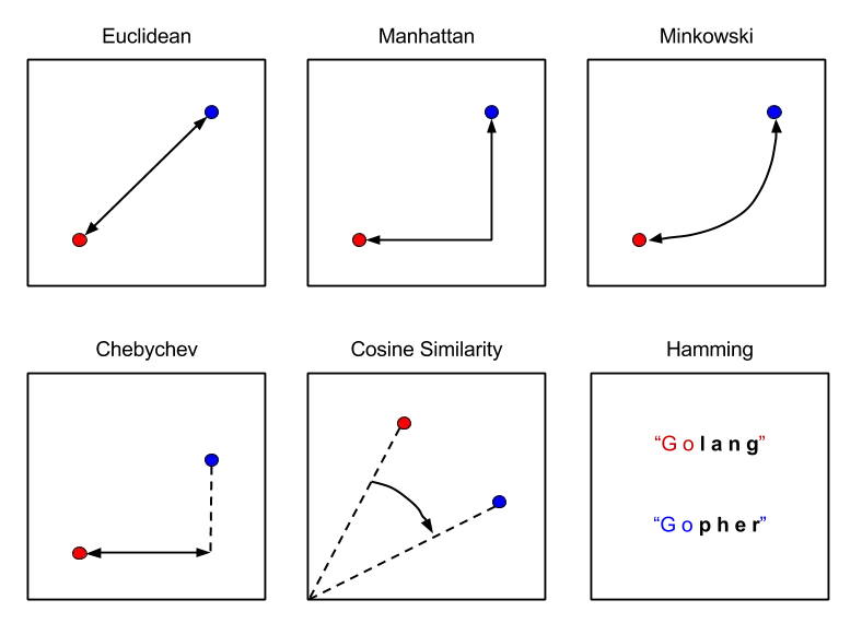
One of the key components of the k-nearest neighbor algorithm is the distance metric used to measure the similarity between two data points. The most commonly used distance metrics are:

Find out more (here)

• Euclidean distance: this is the straight-line distance between two points in Euclidean space. The formula for Euclidean distance between two points, x and y, is:

  \[ d(x,y) = \sqrt {\sum(x_i - y_i)^2} \]

  d(x, y) = sqrt(sum((xi - yi)^2))

• Manhattan distance: this is the distance between two points measured along the axes at right angles. The formula for Manhattan distance between two points, x and y, is:

  \[ d(x,y) = \sum|x_i - y_i| \]

  d(x, y) = sum(|xi - yi|)

• Minkowski distance: this is a generalization of Euclidean and Manhattan distance that allows us to control the “shape” of the distance metric. The formula for Minkowski distance between two points, x and y, is:

  \[ d(x,y) = (\sum|x_i - y_i|^p)^\frac{1}{p} \]

  d(x, y) = (sum(|xi - yi|^p))^(1/p)

  where p is a parameter that controls the “shape” of the distance metric. When p=1, the Minkowski distance is equivalent to Manhattan distance, and when p=2, the Minkowski distance is equivalent to Euclidean distance.

Choosing the right distance metric is important for accurate predictions in the k-nearest neighbor algorithm. You should choose a distance metric that is appropriate for your data and the problem you are trying to solve.

Choosing the value of k

Another important component of the k-nearest neighbor algorithm is the value of k, which represents the number of nearest neighbors used to make the prediction. Choosing the right value of k is crucial for the performance of the algorithm.

If k is too small, the algorithm may be too sensitive to noise and outliers in the data, leading to overfitting. On the other hand, if k is too large, the algorithm may be too general and fail to capture the nuances of the data, leading to underfitting.

One common approach to choosing the value of k is to use cross-validation to evaluate the performance of the algorithm on different values of k and choose the value that gives the best performance.

Weighted versus unweighted k-nearest neighbor algorithm

In the basic k-nearest neighbor algorithm, all k nearest neighbors are treated equally when making the prediction. However, in some cases, it may be more appropriate to assign different weights to the nearest neighbors based on their distance from the new data point.

For example, you may want to give more weight to the nearest neighbors that are closer to the new data point and less weight to the neighbors that are farther away. This can be done by using a weighted k-nearest neighbor algorithm, where the weights are inversely proportional to the distance between the neighbors and the new data point.

Handling ties in k-nearest neighbor algorithm

In some cases, there may be a tie in the labels of the k nearest neighbors, making it difficult to make a prediction. For example, if k=4 and two neighbors are labeled as class A and also two neighbors are labeled as class B, there is a tie between class A and class B.

There are several ways to handle ties in the k-nearest neighbor algorithm. One common approach is to assign the new data point to the class that has the nearest neighbor among the tied classes.

---

Implementation

We introduced the k-nearest neighbor algorithm and discussed its theory, including distance metrics, choosing the value of k, weighted versus unweighted k-nearest neighbor algorithm, and handling ties in k-nearest neighbor algorithm. Let’s learn how to implement the k-nearest neighbor algorithm in R, step by step.

Loading data into R

The first step in implementing the k-nearest neighbor algorithm is to load the data into R. In this example, we’ll use the iris dataset, which contains measurements of iris flowers.

data(iris)

Splitting data into training and testing sets

The next step is to split the data into training and testing sets. We’ll use 70% of the data for training and 30% of the data for testing.

set.seed(123)
train_index <- sample(nrow(iris), 0.7 * nrow(iris))
train_data <- iris[train_index, ]
test_data <- iris[-train_index, ]

Preprocessing data: scaling and centering

Before applying the k-nearest neighbor algorithm, it’s important to preprocess the data by scaling and centering the features. We’ll use the scale function in R to scale and center the data.

train_data_scaled <- scale(train_data[, -5])
test_data_scaled <- scale(test_data[, -5])


head(train_data_scaled)

    Sepal.Length Sepal.Width Petal.Length Petal.Width
14   -1.76664631  -0.1186139   -1.4793538  -1.4471163
50   -0.96560680   0.5607204   -1.3126884  -1.3157877
118   2.12411700   1.6929443    1.6317336   1.3107847
43   -1.65221209   0.3342756   -1.3682435  -1.3157877
150   0.06430113  -0.1186139    0.7428515   0.7854702
148   0.75090642  -0.1186139    0.7984066   1.0481275

summary(train_data_scaled)

  Sepal.Length       Sepal.Width       Petal.Length      Petal.Width     
 Min.   :-1.76665   Min.   :-1.9302   Min.   :-1.5349   Min.   :-1.4471  
 1st Qu.:-0.85117   1st Qu.:-0.5715   1st Qu.:-1.2016   1st Qu.:-1.1845  
 Median :-0.05013   Median :-0.1186   Median : 0.3540   Median : 0.2602  
 Mean   : 0.00000   Mean   : 0.0000   Mean   : 0.0000   Mean   : 0.0000  
 3rd Qu.: 0.63647   3rd Qu.: 0.7872   3rd Qu.: 0.7429   3rd Qu.: 0.7855  
 Max.   : 2.35299   Max.   : 3.0516   Max.   : 1.7428   Max.   : 1.7048  

When working with machine learning algorithms, especially distance-based methods such as k-nearest neighbors (kNN), it is crucial to preprocess the data by scaling and centering the features. This ensures that all features contribute equally to the model’s performance and prevents features with larger magnitudes from dominating the algorithm.

Scaling and centering involve transforming the data such that the features have a mean of 0 and a standard deviation of 1. The transformation is performed using the following equations:

1. Centering (Mean subtraction):

   X_centered = X - mean(X)

   This step involves subtracting the mean of the feature from each data point, effectively centering the data around 0.

2. Scaling (Divide by standard deviation):

   X_scaled = X_centered / sd(X)

   In this step, we divide the centered data by the standard deviation, resulting in a transformed feature with a standard deviation of 1.

In R, we can use the scale() function to perform both centering and scaling in one step. Here’s how to apply it to the train_data and test_data.

Min-max normalization is another preprocessing technique used to scale the features within a specific range, usually [0, 1]. This method can be particularly useful when working with algorithms sensitive to feature magnitudes or when we want to maintain the same unit of measurement across features.

Min-max normalization is performed using the following equation:

X_normalized = (X - min(X)) / (max(X) - min(X))

This transformation scales the data linearly between the minimum and maximum values of each feature.

# Define the min-max normalization function
min_max_normalize <- function(x) {
  (x - min(x)) / (max(x) - min(x))
}

train_data_normalized <- min_max_normalize(train_data[, -5])

head(train_data_normalized)

    Sepal.Length Sepal.Width Petal.Length Petal.Width
14     0.5384615   0.3717949    0.1282051  0.00000000
50     0.6282051   0.4102564    0.1666667  0.01282051
118    0.9743590   0.4743590    0.8461538  0.26923077
43     0.5512821   0.3974359    0.1538462  0.01282051
150    0.7435897   0.3717949    0.6410256  0.21794872
148    0.8205128   0.3717949    0.6538462  0.24358974

summary(train_data_normalized)

  Sepal.Length     Sepal.Width      Petal.Length     Petal.Width     
 Min.   :0.5385   Min.   :0.2692   Min.   :0.1154   Min.   :0.00000  
 1st Qu.:0.6410   1st Qu.:0.3462   1st Qu.:0.1923   1st Qu.:0.02564  
 Median :0.7308   Median :0.3718   Median :0.5513   Median :0.16667  
 Mean   :0.7364   Mean   :0.3785   Mean   :0.4696   Mean   :0.14127  
 3rd Qu.:0.8077   3rd Qu.:0.4231   3rd Qu.:0.6410   3rd Qu.:0.21795  
 Max.   :1.0000   Max.   :0.5513   Max.   :0.8718   Max.   :0.30769  

Writing a function to calculate distances

Next, we’ll write a function to calculate distances between two data points using the Euclidean distance metric.

euclidean_distance <- function(x, y) {
  sqrt(sum((x - y)^2))
}

Implementing k-nearest neighbor algorithm using class package

We’ll use the class package in R to implement the k-nearest neighbor algorithm. We’ll use the knn function in the class package to make predictions based on the k nearest neighbors.

library(class)
k <- 5
predicted_classes <- knn(train = train_data_scaled, 
                         test = test_data_scaled, 
                         cl = train_data[, 5], 
                         k = k, 
                         prob = TRUE)

In the code above, we set k to 5, which means we’ll use the 5 nearest neighbors to make the prediction. The knn function returns the predicted classes of the test data, based on the labels of the nearest neighbors in the training data. The option cl means class, prop means that the result comes with the probability.

Evaluating model performance using confusion matrix, accuracy, precision, recall, and F1-score

Finally, we’ll evaluate the performance of the k-nearest neighbor algorithm using a confusion matrix, accuracy, precision, recall, and F1-score.

library(caret)

Loading required package: ggplot2

Loading required package: lattice

confusion_matrix <- confusionMatrix(predicted_classes, test_data[, 5])
confusion_matrix

Confusion Matrix and Statistics

            Reference
Prediction   setosa versicolor virginica
  setosa         14          0         0
  versicolor      0         17         0
  virginica       0          1        13

Overall Statistics
                                          
               Accuracy : 0.9778          
                 95% CI : (0.8823, 0.9994)
    No Information Rate : 0.4             
    P-Value [Acc > NIR] : < 2.2e-16       
                                          
                  Kappa : 0.9664          
                                          
 Mcnemar's Test P-Value : NA              

Statistics by Class:

                     Class: setosa Class: versicolor Class: virginica
Sensitivity                 1.0000            0.9444           1.0000
Specificity                 1.0000            1.0000           0.9688
Pos Pred Value              1.0000            1.0000           0.9286
Neg Pred Value              1.0000            0.9643           1.0000
Prevalence                  0.3111            0.4000           0.2889
Detection Rate              0.3111            0.3778           0.2889
Detection Prevalence        0.3111            0.3778           0.3111
Balanced Accuracy           1.0000            0.9722           0.9844

confusion_matrix$byClass[,"Precision"]

    Class: setosa Class: versicolor  Class: virginica 
        1.0000000         1.0000000         0.9285714 

confusion_matrix$byClass[,"Recall"]

    Class: setosa Class: versicolor  Class: virginica 
        1.0000000         0.9444444         1.0000000 

confusion_matrix$byClass[,"F1"]

    Class: setosa Class: versicolor  Class: virginica 
        1.0000000         0.9714286         0.9629630 

In the code above, we use the confusionMatrix function in the caret package to generate a confusion matrix based on the predicted classes and the true labels of the test data. We then extract the overall accuracy and the precision, recall, and F1-score for each class from the confusion matrix.

What is F1 score?

F1 score is a measure of a machine learning algorithm’s accuracy that combines precision and recall. It is the harmonic mean of precision and recall, and ranges from 0 to 1, with higher values indicating better performance.

F1 score is calculated using the following formula:

\[ F1 = 2 \times \frac{Precision \times Recall}{Precesion + Recall} \]

F1 score = 2 * (precision * recall) / (precision + recall)

where precision is the number of true positives divided by the total number of positive predictions, and recall is the number of true positives divided by the total number of actual positives.

Why use F1 score?

F1 score is useful when the dataset is imbalanced, meaning that the number of positive and negative examples is not equal. In such cases, accuracy alone is not a good measure of the algorithm’s performance, as a high accuracy can be achieved by simply predicting the majority class all the time.

Instead, we need a metric that takes into account both precision and recall, as precision measures the algorithm’s ability to make correct positive predictions, and recall measures the algorithm’s ability to find all positive examples in the dataset.

How to interpret F1 score?

F1 score ranges from 0 to 1, with higher values indicating better performance. An F1 score of 1 means perfect precision and recall, while an F1 score of 0 means that either the precision or recall is 0.

In practice, we aim to achieve a high F1 score while balancing precision and recall based on the problem and its requirements. For example, in medical diagnosis, we may want to prioritize recall over precision to avoid missing any positive cases, while in fraud detection, we may want to prioritize precision over recall to avoid false positives.

---

QZs

1. Which of the following is a distance metric commonly used in the k-nearest neighbor algorithm?
   1. Correlation distance
   2. Chebyshev distance
   3. Hamming distance
   4. All of the above
2. How do you choose the value of k in the k-nearest neighbor algorithm?
   1. Choose a small value of k to avoid overfitting
   2. Choose a large value of k to avoid overfitting
   3. Use cross-validation to evaluate the performance of the algorithm on different values of k and choose the value that gives the best performance
   4. None of the above
3. What is the difference between weighted and unweighted k-nearest neighbor algorithm?
   1. Weighted k-nearest neighbor algorithm gives more weight to the nearest neighbors that are farther away
   2. Unweighted k-nearest neighbor algorithm gives more weight to the nearest neighbors that are closer
   3. Weighted k-nearest neighbor algorithm assigns different weights to the nearest neighbors based on their distance from the new data point
   4. Unweighted k-nearest neighbor algorithm assigns different weights to the nearest neighbors based on their distance from the new data point
4. What is F1 score?
   1. A measure of a machine learning algorithm’s accuracy that combines precision and recall
   2. The average of precision and recall
   3. The harmonic mean of precision and recall
   4. None of the above
5. What is the formula for calculating Euclidean distance between two points in Euclidean space?
   1. d(x, y) = sqrt(sum((xi - yi)^2))
   2. d(x, y) = sum(|xi - yi|)
   3. d(x, y) = (sum(|xi - yi|^p))^(1/p)
   4. None of the above
6. What is the purpose of scaling and centering the features in the k-nearest neighbor algorithm?
   1. To make the features easier to interpret
   2. To make the features more accurate
   3. To make the features more comparable
   4. None of the above
7. How can you handle ties in the k-nearest neighbor algorithm?
   1. Assign the new data point to the class that has the nearest neighbor among the tied classes
   2. Assign the new data point to the class that has the farthest neighbor among the tied classes
   3. Assign the new data point to the class that has the most neighbors among the tied classes
   4. None of the above

Ans) dcccaca

---

In this week, we learned about the k-nearest neighbor algorithm, a popular machine learning algorithm used for classification and regression problems. We started with an overview of the algorithm and its applications, and discussed the advantages and disadvantages of the algorithm.

We then delved into the theory behind the k-nearest neighbor algorithm, including distance metrics such as Euclidean distance and Manhattan distance, choosing the value of k, weighted versus unweighted k-nearest neighbor algorithm, and handling ties in k-nearest neighbor algorithm.

We also showed you how to implement the k-nearest neighbor algorithm in R step by step, including loading data into R, splitting data into training and testing sets, preprocessing data, writing a function to calculate distances, and evaluating model performance using confusion matrix, accuracy, precision, recall, and F1-score.

Finally, we gave you the opportunity to practice implementing the k-nearest neighbor algorithm on your own data set and evaluate the model’s performance.

By understanding the k-nearest neighbor algorithm and its theory, as well as its implementation in R, you can apply this algorithm to your own machine learning problems and make informed decisions about your data. Keep practicing and exploring different machine learning algorithms to expand your knowledge and skills in data science.

---

Model Comparison with tidymodels in R

Let’s learn how to compare four different machine learning models using the tidymodels package in R. We will be using the classic Iris dataset to showcase this comparison. The models we will compare are Decision Trees, Random Forests, Naive Bayes, and k-Nearest Neighbors (kNN).

First, let’s load the necessary libraries and the Iris dataset.

# Load the required libraries
library(tidymodels)

── Attaching packages ────────────────────────────────────── tidymodels 1.2.0 ──

✔ broom        1.0.6     ✔ rsample      1.2.1
✔ dials        1.3.0     ✔ tibble       3.2.1
✔ dplyr        1.1.4     ✔ tidyr        1.3.1
✔ infer        1.0.7     ✔ tune         1.2.1
✔ modeldata    1.4.0     ✔ workflows    1.1.4
✔ parsnip      1.2.1     ✔ workflowsets 1.1.0
✔ purrr        1.0.2     ✔ yardstick    1.3.1
✔ recipes      1.1.0     

── Conflicts ───────────────────────────────────────── tidymodels_conflicts() ──
✖ purrr::discard()         masks scales::discard()
✖ dplyr::filter()          masks stats::filter()
✖ dplyr::lag()             masks stats::lag()
✖ purrr::lift()            masks caret::lift()
✖ yardstick::precision()   masks caret::precision()
✖ yardstick::recall()      masks caret::recall()
✖ yardstick::sensitivity() masks caret::sensitivity()
✖ yardstick::specificity() masks caret::specificity()
✖ recipes::step()          masks stats::step()
• Search for functions across packages at https://www.tidymodels.org/find/

library(tidyverse)

── Attaching core tidyverse packages ──────────────────────── tidyverse 2.0.0 ──
✔ forcats   1.0.0     ✔ readr     2.1.5
✔ lubridate 1.9.3     ✔ stringr   1.5.1

── Conflicts ────────────────────────────────────────── tidyverse_conflicts() ──
✖ readr::col_factor() masks scales::col_factor()
✖ purrr::discard()    masks scales::discard()
✖ dplyr::filter()     masks stats::filter()
✖ stringr::fixed()    masks recipes::fixed()
✖ dplyr::lag()        masks stats::lag()
✖ purrr::lift()       masks caret::lift()
✖ readr::spec()       masks yardstick::spec()
ℹ Use the conflicted package (<http://conflicted.r-lib.org/>) to force all conflicts to become errors

library(rpart)

Attaching package: 'rpart'

The following object is masked from 'package:dials':

    prune

library(rpart.plot)
library(discrim)

Attaching package: 'discrim'

The following object is masked from 'package:dials':

    smoothness

library(naivebayes)

naivebayes 1.0.0 loaded
For more information please visit: 
https://majkamichal.github.io/naivebayes/

library(kknn)

Attaching package: 'kknn'

The following object is masked from 'package:caret':

    contr.dummy

library(yardstick)

# Load the Iris dataset
data(iris)

Before we begin modeling, we need to preprocess the data. We will split the dataset into training (75%) and testing (25%) sets.

# Split the data into training and testing sets
set.seed(42)
data_split <- initial_split(iris, prop = 0.75)
train_data <- training(data_split)
test_data <- testing(data_split)

Now, we will create the models using tidymodels’ parsnip package. Each model will be created using a similar structure, specifying the model type and the mode (classification in this case).

# Decision Tree
decision_tree <- decision_tree() %>%
  set_engine("rpart") %>%
  set_mode("classification")

# Random Forest
random_forest <- rand_forest() %>%
  set_engine("randomForest") %>%
  set_mode("classification")

# Naive Bayes
naive_bayes <- naive_Bayes() %>%
  set_engine("naivebayes") %>%
  set_mode("classification")

# k-Nearest Neighbors (kNN)
knn <- nearest_neighbor() %>%
  set_engine("kknn") %>%
  set_mode("classification")

Next, we will create a workflow for each model. In this example, we don’t require any preprocessing steps, so we will directly specify the model in the workflow.

# Decision Tree Workflow
workflow_dt <- workflow() %>%
  add_model(decision_tree) %>%
  add_formula(Species ~ .)


# Random Forest Workflow
workflow_rf <- workflow() %>%
  add_model(random_forest) %>%
  add_formula(Species ~ .)

# Naive Bayes Workflow
workflow_nb <- workflow() %>%
  add_model(naive_bayes) %>%
  add_formula(Species ~ .)

# kNN Workflow
workflow_knn <- workflow() %>%
  add_model(knn) %>%
  add_formula(Species ~ .)

We will now fit each model using the training data and make predictions on the test data.

# Fit the models
fit_dt <- fit(workflow_dt, data = train_data)
fit_rf <- fit(workflow_rf, data = train_data)
fit_nb <- fit(workflow_nb, data = train_data)
fit_knn <- fit(workflow_knn, data = train_data)

Finally, we will evaluate the performance of each model using accuracy as the metric.

predict(fit_dt, test_data) %>% 
  bind_cols(predict(fit_dt, test_data, type = "prob")) %>% 
  # Add the true outcome data back in
  bind_cols(test_data %>% 
              select(Species))

# A tibble: 38 × 5
   .pred_class .pred_setosa .pred_versicolor .pred_virginica Species
   <fct>              <dbl>            <dbl>           <dbl> <fct>  
 1 setosa                 1                0               0 setosa 
 2 setosa                 1                0               0 setosa 
 3 setosa                 1                0               0 setosa 
 4 setosa                 1                0               0 setosa 
 5 setosa                 1                0               0 setosa 
 6 setosa                 1                0               0 setosa 
 7 setosa                 1                0               0 setosa 
 8 setosa                 1                0               0 setosa 
 9 setosa                 1                0               0 setosa 
10 setosa                 1                0               0 setosa 
# ℹ 28 more rows

predict(fit_dt, test_data) %>% 
  bind_cols(predict(fit_dt, test_data, type = "prob")) %>% 
  bind_cols(test_data %>% 
              select(Species)) %>% 
  # Add accuracy function from yardstick
  accuracy(truth = Species, .pred_class)

# A tibble: 1 × 3
  .metric  .estimator .estimate
  <chr>    <chr>          <dbl>
1 accuracy multiclass     0.947

# All together 
accuracy_dt <- 
  predict(fit_dt, test_data) %>% 
  bind_cols(predict(fit_dt, test_data, type = "prob")) %>% 
  bind_cols(test_data %>% 
              select(Species)) %>% 
  accuracy(truth = Species, .pred_class)

Do the same things for the other models

accuracy_rf <- 
  predict(fit_rf, test_data) %>% 
  bind_cols(predict(fit_rf, test_data, type = "prob")) %>% 
  bind_cols(test_data %>% 
              select(Species)) %>% 
  accuracy(truth = Species, .pred_class)

accuracy_nb <- 
  predict(fit_nb, test_data) %>% 
  bind_cols(predict(fit_nb, test_data, type = "prob")) %>% 
  bind_cols(test_data %>% 
              select(Species)) %>% 
  accuracy(truth = Species, .pred_class)

accuracy_knn <- 
  predict(fit_knn, test_data) %>% 
  bind_cols(predict(fit_knn, test_data, type = "prob")) %>% 
  bind_cols(test_data %>% 
              select(Species)) %>% 
  accuracy(truth = Species, .pred_class)

calculates the accuracy for each model and displays the results in a sorted data frame.

accuracy_dt %>% 
  bind_rows(accuracy_rf, accuracy_nb, accuracy_knn) %>% 
  mutate(models = c("Decision Tree", "Random Forest", "Naive Bayes", "kNN")) %>% 
  arrange(desc(.estimate))

# A tibble: 4 × 4
  .metric  .estimator .estimate models       
  <chr>    <chr>          <dbl> <chr>        
1 accuracy multiclass     0.974 kNN          
2 accuracy multiclass     0.947 Decision Tree
3 accuracy multiclass     0.947 Random Forest
4 accuracy multiclass     0.947 Naive Bayes