Unsupervised Learning

Pattern Finding

Weekly design


Pre-class video

  • Eng ver.
  • Kor ver.
  • Pre-class PPT pdf

Discussion

Discussion #9


Class

Apriori Algorithm Implementation in R using ‘arules’ library Association mining is usually done on transactions data from a retail market or from an online e-commerce store. Since most transactions data is large, the apriori algorithm makes it easier to find these patterns or rules quickly. Association Rules are widely used to analyze retail basket or transaction data, and are intended to identify strong rules discovered in transaction data using measures of interestingness, based on the concept of strong rules.

Apriori uses a “bottom up” approach, where frequent subsets are extended one item at a time (a step known as candidate generation), and groups of candidates are tested against the data. The algorithm terminates when no further successful extensions are found.


Download the grocery dataset

[Grocery data]

Import Required libraries and data

library(tidyverse)
── Attaching core tidyverse packages ──────────────────────── tidyverse 2.0.0 ──
✔ dplyr     1.1.4     ✔ readr     2.1.5
✔ forcats   1.0.0     ✔ stringr   1.5.1
✔ ggplot2   3.5.1     ✔ tibble    3.2.1
✔ lubridate 1.9.3     ✔ tidyr     1.3.1
✔ purrr     1.0.2     
── Conflicts ────────────────────────────────────────── tidyverse_conflicts() ──
✖ dplyr::filter() masks stats::filter()
✖ dplyr::lag()    masks stats::lag()
ℹ Use the conflicted package (<http://conflicted.r-lib.org/>) to force all conflicts to become errors
library(plyr)
------------------------------------------------------------------------------
You have loaded plyr after dplyr - this is likely to cause problems.
If you need functions from both plyr and dplyr, please load plyr first, then dplyr:
library(plyr); library(dplyr)
------------------------------------------------------------------------------

Attaching package: 'plyr'

The following objects are masked from 'package:dplyr':

    arrange, count, desc, failwith, id, mutate, rename, summarise,
    summarize

The following object is masked from 'package:purrr':

    compact
groceries <- read.csv("content/Groceries_dataset.csv")
head(groceries, 20)
   Member_number       Date           itemDescription
1           1808 21-07-2015            tropical fruit
2           2552 05-01-2015                whole milk
3           2300 19-09-2015                 pip fruit
4           1187 12-12-2015          other vegetables
5           3037 01-02-2015                whole milk
6           4941 14-02-2015                rolls/buns
7           4501 08-05-2015          other vegetables
8           3803 23-12-2015                pot plants
9           2762 20-03-2015                whole milk
10          4119 12-02-2015            tropical fruit
11          1340 24-02-2015              citrus fruit
12          2193 14-04-2015                      beef
13          1997 21-07-2015               frankfurter
14          4546 03-09-2015                   chicken
15          4736 21-07-2015                    butter
16          1959 30-03-2015     fruit/vegetable juice
17          1974 03-05-2015 packaged fruit/vegetables
18          2421 02-09-2015                 chocolate
19          1513 03-08-2015             specialty bar
20          1905 07-07-2015          other vegetables

Data Cleaning and Exploration

Checking NA values

glimpse(groceries)
Rows: 38,765
Columns: 3
$ Member_number   <int> 1808, 2552, 2300, 1187, 3037, 4941, 4501, 3803, 2762, …
$ Date            <chr> "21-07-2015", "05-01-2015", "19-09-2015", "12-12-2015"…
$ itemDescription <chr> "tropical fruit", "whole milk", "pip fruit", "other ve…
summary(groceries)
 Member_number      Date           itemDescription   
 Min.   :1000   Length:38765       Length:38765      
 1st Qu.:2002   Class :character   Class :character  
 Median :3005   Mode  :character   Mode  :character  
 Mean   :3004                                        
 3rd Qu.:4007                                        
 Max.   :5000                                        
sum(is.na(groceries))
[1] 0

Group all the items that were bought together by the same customer on the same date

itemList <- ddply(groceries, 
                  c("Member_number","Date"), 
                  function(df1) paste(df1$itemDescription, collapse = ",")
                  )
                  
head(itemList,15)
   Member_number       Date                                            V1
1           1000 15-03-2015 sausage,whole milk,semi-finished bread,yogurt
2           1000 24-06-2014                 whole milk,pastry,salty snack
3           1000 24-07-2015                   canned beer,misc. beverages
4           1000 25-11-2015                      sausage,hygiene articles
5           1000 27-05-2015                       soda,pickled vegetables
6           1001 02-05-2015                              frankfurter,curd
7           1001 07-02-2014                 sausage,whole milk,rolls/buns
8           1001 12-12-2014                               whole milk,soda
9           1001 14-04-2015                              beef,white bread
10          1001 20-01-2015           frankfurter,soda,whipped/sour cream
11          1002 09-02-2014            frozen vegetables,other vegetables
12          1002 26-04-2014                             butter,whole milk
13          1002 26-04-2015                          tropical fruit,sugar
14          1002 30-08-2015               butter milk,specialty chocolate
15          1003 10-02-2015                            sausage,rolls/buns

Remove member number and date

itemList %>% 
  select(V1) %>% 
  setNames(c("itemList")) %>% 
  head
                                       itemList
1 sausage,whole milk,semi-finished bread,yogurt
2                 whole milk,pastry,salty snack
3                   canned beer,misc. beverages
4                      sausage,hygiene articles
5                       soda,pickled vegetables
6                              frankfurter,curd
itemList <- itemList %>% 
  select(V1) %>% 
  setNames(c("itemList")) 

write.csv(itemList,"ItemList.csv", quote = FALSE, row.names = TRUE)

Convert CSV file to Basket Format

library(arules)
Loading required package: Matrix

Attaching package: 'Matrix'
The following objects are masked from 'package:tidyr':

    expand, pack, unpack

Attaching package: 'arules'
The following object is masked from 'package:dplyr':

    recode
The following objects are masked from 'package:base':

    abbreviate, write
library(arulesViz)
# read the transactional dataset from a CSV file and convert it into a transaction object
txn = read.transactions(file = "ItemList.csv", 
                         rm.duplicates = TRUE, # remove duplicate transactions
                         format = "basket", # dataset is in basket format (each row represents a single transaction)
                         sep = ",", # CSV file is comma-separated
                         cols = 1) # transaction IDs are stored in the first column of the CSV file
distribution of transactions with duplicates:
items
  1   2   3   4 
662  39   5   1 
print(txn)
transactions in sparse format with
 14964 transactions (rows) and
 168 items (columns)


  1. The first line of output shows the distribution of transactions by item. In this case, there are four items (items 1, 2, 3, and 4), and the numbers indicate how many transactions in the dataset contain each item. For example, there are 662 transactions that contain item 1, 39 transactions that contain item 2, 5 transactions that contain item 3, and 1 transaction that contains item 4. This information is useful for understanding the frequency of different items in the dataset and identifying which items are most commonly associated with each other.

  2. The second line of output shows the total number of transactions in the dataset and the number of unique items that appear in those transactions. Specifically, there are 14964 transactions (rows) and 168 unique items (columns). The transactions are in sparse format, meaning that the majority of the entries in the transaction matrix are zero (i.e., most transactions do not contain most of the items). This format is used to save memory when working with large datasets that have many items.


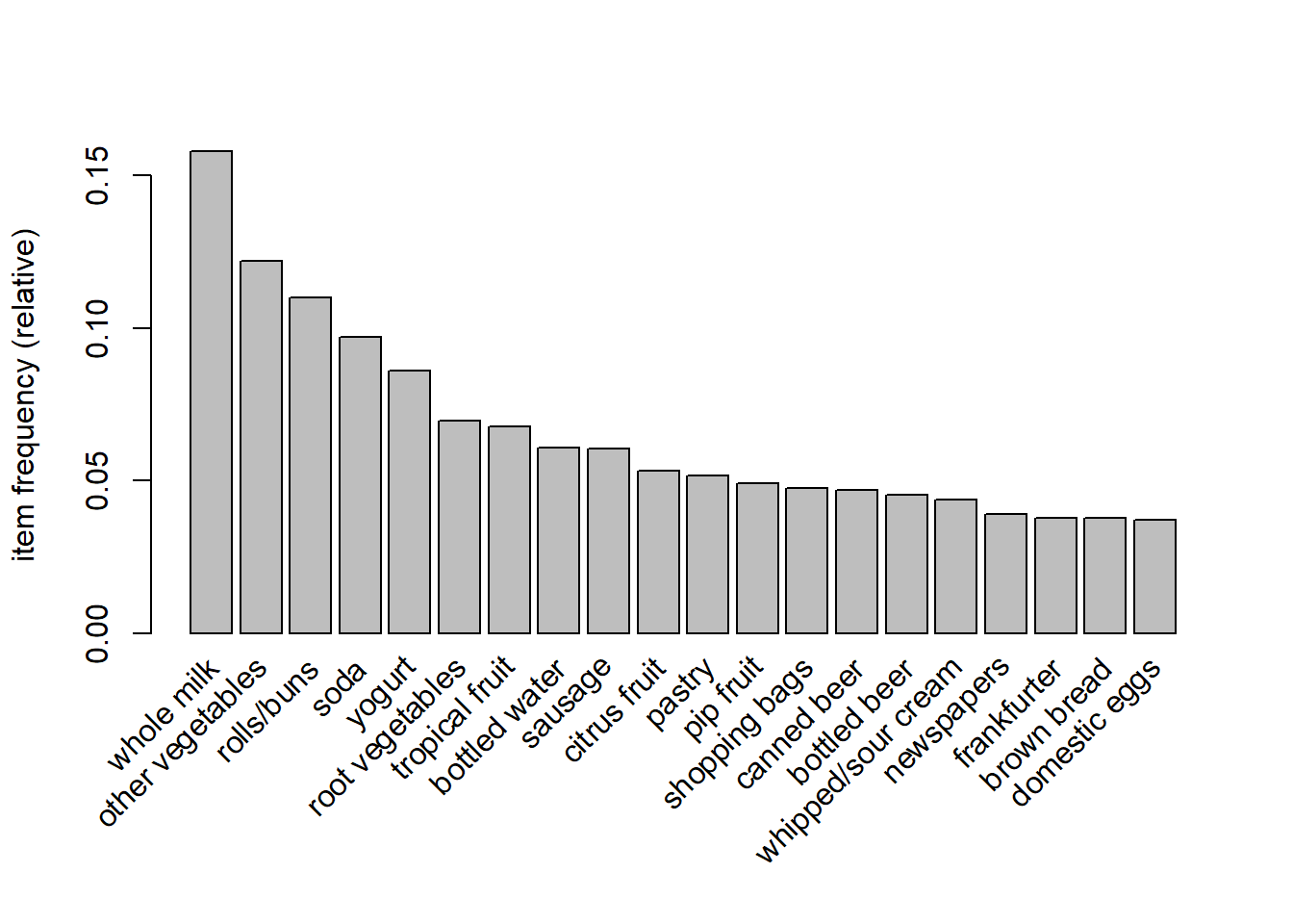
Most Frequent Products

itemFrequencyPlot(txn, topN = 20)

Apriori Algorithm The apriori() generates the most relevent set of rules from a given transaction data. It also shows the support, confidence and lift of those rules. These three measure can be used to decide the relative strength of the rules. So what do these terms mean?

Lets consider the rule {X → Y} in order to compute these metrics.

\[ Support(X,Y) = \frac{frq(X,Y)}{N} \]

\[ Confidence(X → Y) = \frac{frq(X,Y)}{frq(X)} \]

\[ Lift(X → Y) = \frac{Confidence(X → Y)}{Support(Y)} \]


basket_rules <- apriori(txn, 
                        parameter = list(
                          minlen = 2, # Minimum number of items in a rule (in this case, 2)
                          sup = 0.001, # Minimum support threshold (a rule must be present in at least 0.1% of transactions)
                          conf = 0.05, # Minimum confidence threshold (rules must have at least 5% confidence)
                          target = "rules" # Specifies that we want to generate association rules
                        ))
Apriori

Parameter specification:
 confidence minval smax arem  aval originalSupport maxtime support minlen
       0.05    0.1    1 none FALSE            TRUE       5   0.001      2
 maxlen target  ext
     10  rules TRUE

Algorithmic control:
 filter tree heap memopt load sort verbose
    0.1 TRUE TRUE  FALSE TRUE    2    TRUE

Absolute minimum support count: 14 

set item appearances ...[0 item(s)] done [0.00s].
set transactions ...[168 item(s), 14964 transaction(s)] done [0.00s].
sorting and recoding items ... [149 item(s)] done [0.00s].
creating transaction tree ... done [0.00s].
checking subsets of size 1 2 3 4 done [0.00s].
writing ... [450 rule(s)] done [0.00s].
creating S4 object  ... done [0.00s].

The apriori function takes several parameters, including the transaction dataset (txn) and a list of parameters (parameter) that control the behavior of the algorithm. The minlen parameter sets the minimum number of items in a rule to 2, which means that the algorithm will only consider rules that involve at least 2 items. The sup parameter sets the minimum support threshold to 0.001, which means that a rule must be present in at least 0.1% of transactions in order to be considered significant. The conf parameter sets the minimum confidence threshold to 0.05, which means that a rule must have at least 5% confidence (i.e., be correct at least 5% of the time) to be considered significant. Finally, the target parameter specifies that we want to generate association rules rather than just frequent itemsets.


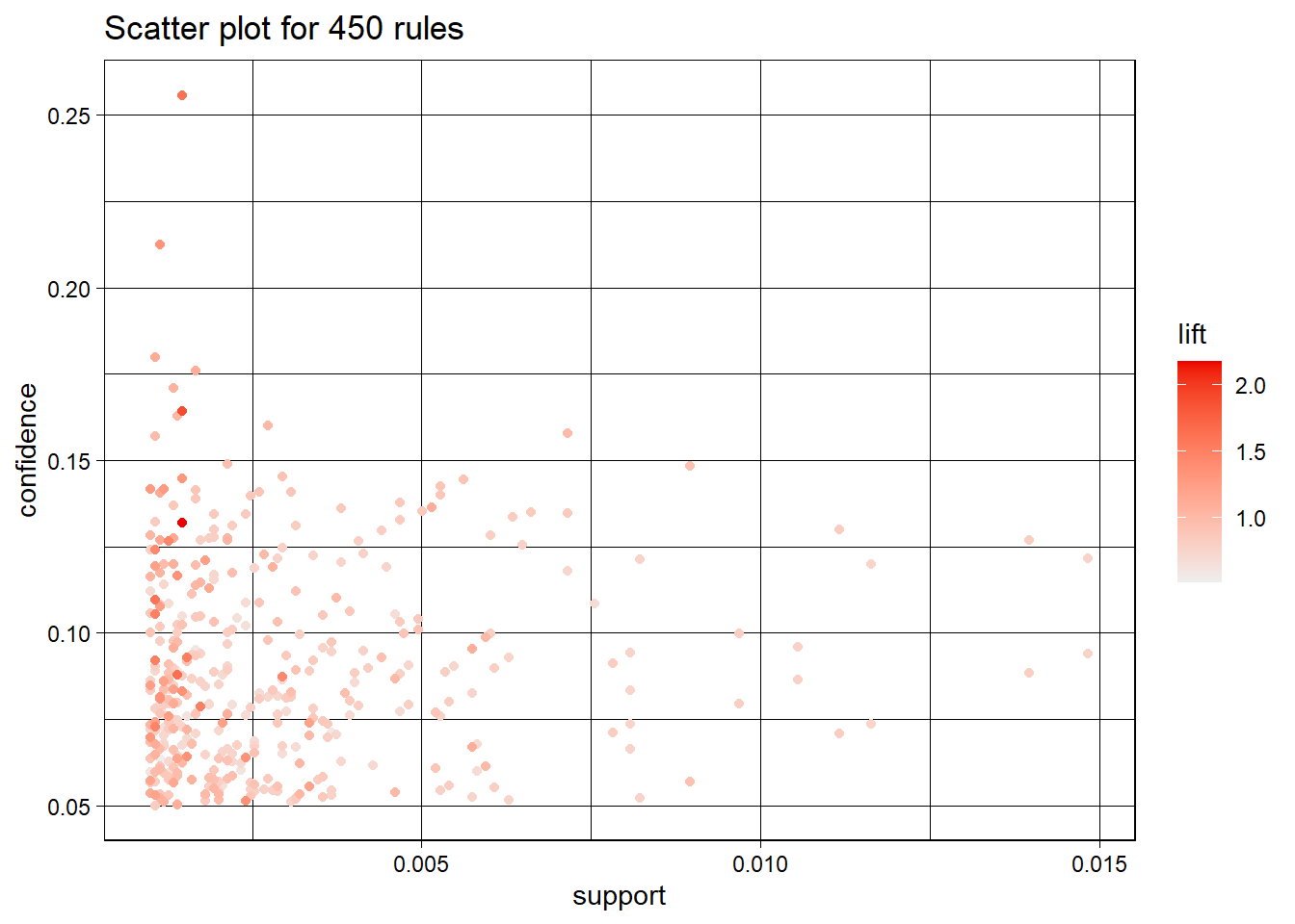
Total rules generated

print(length(basket_rules))
[1] 450
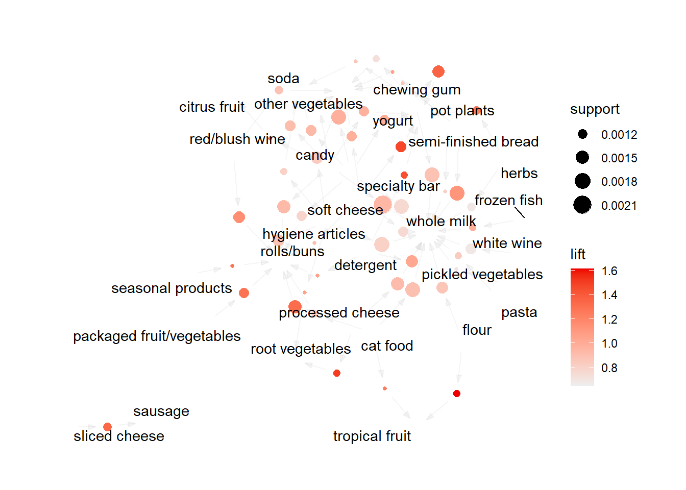
summary(basket_rules)
set of 450 rules

rule length distribution (lhs + rhs):sizes
  2   3 
423  27 

   Min. 1st Qu.  Median    Mean 3rd Qu.    Max. 
   2.00    2.00    2.00    2.06    2.00    3.00 

summary of quality measures:
    support           confidence         coverage             lift       
 Min.   :0.001002   Min.   :0.05000   Min.   :0.005346   Min.   :0.5195  
 1st Qu.:0.001270   1st Qu.:0.06397   1st Qu.:0.015972   1st Qu.:0.7673  
 Median :0.001938   Median :0.08108   Median :0.023590   Median :0.8350  
 Mean   :0.002760   Mean   :0.08759   Mean   :0.033723   Mean   :0.8859  
 3rd Qu.:0.003341   3rd Qu.:0.10482   3rd Qu.:0.043705   3rd Qu.:0.9601  
 Max.   :0.014836   Max.   :0.25581   Max.   :0.157912   Max.   :2.1831  
     count      
 Min.   : 15.0  
 1st Qu.: 19.0  
 Median : 29.0  
 Mean   : 41.3  
 3rd Qu.: 50.0  
 Max.   :222.0  

mining info:
 data ntransactions support confidence
  txn         14964   0.001       0.05
                                                                                          call
 apriori(data = txn, parameter = list(minlen = 2, sup = 0.001, conf = 0.05, target = "rules"))
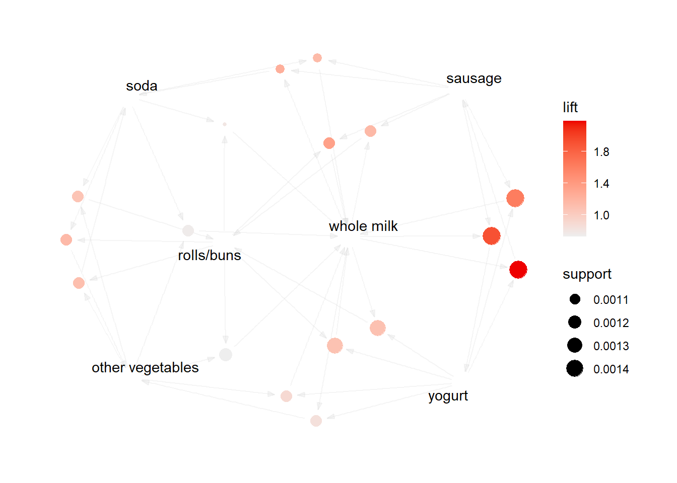
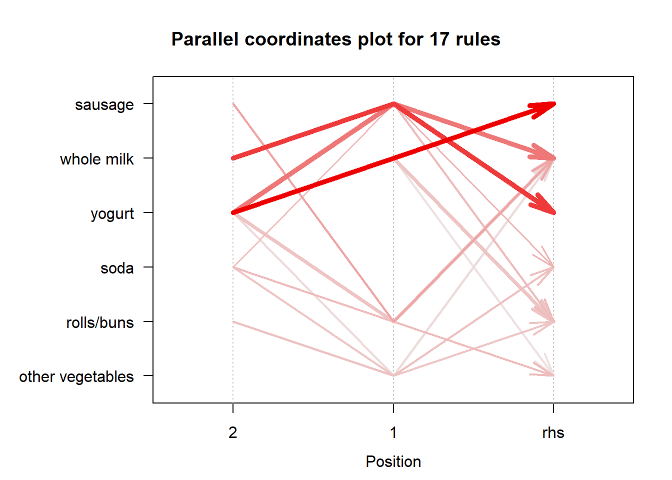
Inspecting the basket rules

inspect(basket_rules[1:20])
     lhs                            rhs                support     confidence
[1]  {frozen fish}               => {whole milk}       0.001069233 0.1568627 
[2]  {seasonal products}         => {rolls/buns}       0.001002406 0.1415094 
[3]  {pot plants}                => {other vegetables} 0.001002406 0.1282051 
[4]  {pot plants}                => {whole milk}       0.001002406 0.1282051 
[5]  {pasta}                     => {whole milk}       0.001069233 0.1322314 
[6]  {pickled vegetables}        => {whole milk}       0.001002406 0.1119403 
[7]  {packaged fruit/vegetables} => {rolls/buns}       0.001202887 0.1417323 
[8]  {detergent}                 => {yogurt}           0.001069233 0.1240310 
[9]  {detergent}                 => {rolls/buns}       0.001002406 0.1162791 
[10] {detergent}                 => {whole milk}       0.001403368 0.1627907 
[11] {semi-finished bread}       => {other vegetables} 0.001002406 0.1056338 
[12] {semi-finished bread}       => {whole milk}       0.001670676 0.1760563 
[13] {red/blush wine}            => {rolls/buns}       0.001336541 0.1273885 
[14] {red/blush wine}            => {other vegetables} 0.001136060 0.1082803 
[15] {flour}                     => {tropical fruit}   0.001069233 0.1095890 
[16] {flour}                     => {whole milk}       0.001336541 0.1369863 
[17] {herbs}                     => {yogurt}           0.001136060 0.1075949 
[18] {herbs}                     => {whole milk}       0.001136060 0.1075949 
[19] {processed cheese}          => {root vegetables}  0.001069233 0.1052632 
[20] {processed cheese}          => {rolls/buns}       0.001470195 0.1447368 
     coverage    lift      count
[1]  0.006816359 0.9933534 16   
[2]  0.007083667 1.2864807 15   
[3]  0.007818765 1.0500611 15   
[4]  0.007818765 0.8118754 15   
[5]  0.008086073 0.8373723 16   
[6]  0.008954825 0.7088763 15   
[7]  0.008487036 1.2885066 18   
[8]  0.008620690 1.4443580 16   
[9]  0.008620690 1.0571081 15   
[10] 0.008620690 1.0308929 21   
[11] 0.009489441 0.8651911 15   
[12] 0.009489441 1.1148993 25   
[13] 0.010491847 1.1581057 20   
[14] 0.010491847 0.8868668 17   
[15] 0.009756750 1.6172489 16   
[16] 0.009756750 0.8674833 20   
[17] 0.010558674 1.2529577 17   
[18] 0.010558674 0.6813587 17   
[19] 0.010157712 1.5131200 16   
[20] 0.010157712 1.3158214 22   

Visualizing the Association Rules

plot(basket_rules, jitter = 0)

plot(basket_rules, method = "grouped", control = list(k = 5))

Graph of first 20 rules

plot(basket_rules[1:20], method="graph")

Graph of first 50 rules

plot(basket_rules[1:50], method="graph")

Parallel coordinates plot

plot(basket_rules[1:20], method="paracoord")

Changing hyperparameters:

basket_rules2 <- apriori(txn, 
                         parameter = list(minlen=3, 
                                          sup = 0.001, 
                                          conf = 0.1,
                                          target="rules"))
Apriori

Parameter specification:
 confidence minval smax arem  aval originalSupport maxtime support minlen
        0.1    0.1    1 none FALSE            TRUE       5   0.001      3
 maxlen target  ext
     10  rules TRUE

Algorithmic control:
 filter tree heap memopt load sort verbose
    0.1 TRUE TRUE  FALSE TRUE    2    TRUE

Absolute minimum support count: 14 

set item appearances ...[0 item(s)] done [0.00s].
set transactions ...[168 item(s), 14964 transaction(s)] done [0.00s].
sorting and recoding items ... [149 item(s)] done [0.00s].
creating transaction tree ... done [0.00s].
checking subsets of size 1 2 3 4 done [0.00s].
writing ... [17 rule(s)] done [0.00s].
creating S4 object  ... done [0.00s].
print(length(basket_rules2))
[1] 17
summary(basket_rules2)
set of 17 rules

rule length distribution (lhs + rhs):sizes
 3 
17 

   Min. 1st Qu.  Median    Mean 3rd Qu.    Max. 
      3       3       3       3       3       3 

summary of quality measures:
    support           confidence        coverage             lift       
 Min.   :0.001002   Min.   :0.1018   Min.   :0.005346   Min.   :0.7214  
 1st Qu.:0.001136   1st Qu.:0.1172   1st Qu.:0.008086   1st Qu.:0.8897  
 Median :0.001136   Median :0.1269   Median :0.008955   Median :1.1081  
 Mean   :0.001207   Mean   :0.1437   Mean   :0.008821   Mean   :1.1794  
 3rd Qu.:0.001337   3rd Qu.:0.1642   3rd Qu.:0.010559   3rd Qu.:1.2297  
 Max.   :0.001470   Max.   :0.2558   Max.   :0.011160   Max.   :2.1831  
     count      
 Min.   :15.00  
 1st Qu.:17.00  
 Median :17.00  
 Mean   :18.06  
 3rd Qu.:20.00  
 Max.   :22.00  

mining info:
 data ntransactions support confidence
  txn         14964   0.001        0.1
                                                                                         call
 apriori(data = txn, parameter = list(minlen = 3, sup = 0.001, conf = 0.1, target = "rules"))
inspect(basket_rules2)
     lhs                               rhs                support    
[1]  {sausage, yogurt}              => {whole milk}       0.001470195
[2]  {sausage, whole milk}          => {yogurt}           0.001470195
[3]  {whole milk, yogurt}           => {sausage}          0.001470195
[4]  {sausage, soda}                => {whole milk}       0.001069233
[5]  {sausage, whole milk}          => {soda}             0.001069233
[6]  {rolls/buns, sausage}          => {whole milk}       0.001136060
[7]  {sausage, whole milk}          => {rolls/buns}       0.001136060
[8]  {rolls/buns, yogurt}           => {whole milk}       0.001336541
[9]  {whole milk, yogurt}           => {rolls/buns}       0.001336541
[10] {other vegetables, yogurt}     => {whole milk}       0.001136060
[11] {whole milk, yogurt}           => {other vegetables} 0.001136060
[12] {rolls/buns, soda}             => {other vegetables} 0.001136060
[13] {other vegetables, soda}       => {rolls/buns}       0.001136060
[14] {other vegetables, rolls/buns} => {soda}             0.001136060
[15] {rolls/buns, soda}             => {whole milk}       0.001002406
[16] {other vegetables, soda}       => {whole milk}       0.001136060
[17] {other vegetables, rolls/buns} => {whole milk}       0.001202887
     confidence coverage    lift      count
[1]  0.2558140  0.005747126 1.6199746 22   
[2]  0.1641791  0.008954825 1.9118880 22   
[3]  0.1317365  0.011160118 2.1830624 22   
[4]  0.1797753  0.005947608 1.1384500 16   
[5]  0.1194030  0.008954825 1.2296946 16   
[6]  0.2125000  0.005346164 1.3456835 17   
[7]  0.1268657  0.008954825 1.1533523 17   
[8]  0.1709402  0.007818765 1.0825005 20   
[9]  0.1197605  0.011160118 1.0887581 20   
[10] 0.1404959  0.008086073 0.8897081 17   
[11] 0.1017964  0.011160118 0.8337610 17   
[12] 0.1404959  0.008086073 1.1507281 17   
[13] 0.1172414  0.009689922 1.0658566 17   
[14] 0.1075949  0.010558674 1.1080872 17   
[15] 0.1239669  0.008086073 0.7850365 15   
[16] 0.1172414  0.009689922 0.7424460 17   
[17] 0.1139241  0.010558674 0.7214386 18   
plot(basket_rules2, method="graph")

plot(basket_rules2, method="paracoord")