Unsupervised Learning

Clustering

Weekly design


Pre-class video

  • Eng ver.
  • Kor ver.
  • Pre-class PPT pdf

Discussion

Discussion #8


Class

K-Means Clustering in R

The basic idea behind k-means clustering consists of defining clusters so that the total intra-cluster variation (known as total within-cluster variation) is minimized. There are several k-means algorithms available. The standard algorithm is the Hartigan-Wong algorithm (Hartigan and Wong 1979), which defines the total within-cluster variation as the sum of squared distances Euclidean distances between items and the corresponding centroid


Let’s experiment with this simple shiny app

https://jjallaire.shinyapps.io/shiny-k-means/


Hands-on practice

Data we’ll use is USArrests. The data must contains only continuous variables, as the k-means algorithm uses variable means.

library(tidyverse)
── Attaching core tidyverse packages ──────────────────────── tidyverse 2.0.0 ──
✔ dplyr     1.1.4     ✔ readr     2.1.5
✔ forcats   1.0.0     ✔ stringr   1.5.1
✔ ggplot2   3.5.1     ✔ tibble    3.2.1
✔ lubridate 1.9.3     ✔ tidyr     1.3.1
✔ purrr     1.0.2     
── Conflicts ────────────────────────────────────────── tidyverse_conflicts() ──
✖ dplyr::filter() masks stats::filter()
✖ dplyr::lag()    masks stats::lag()
ℹ Use the conflicted package (<http://conflicted.r-lib.org/>) to force all conflicts to become errors
data("USArrests")      # Loading the data set
head(USArrests)
           Murder Assault UrbanPop Rape
Alabama      13.2     236       58 21.2
Alaska       10.0     263       48 44.5
Arizona       8.1     294       80 31.0
Arkansas      8.8     190       50 19.5
California    9.0     276       91 40.6
Colorado      7.9     204       78 38.7

The USArrests dataset is a built-in dataset in R that contains data on crime rates (number of arrests per 100,000 residents) in the United States in 1973. The dataset has 50 observations, corresponding to the 50 US states, and 4 variables:

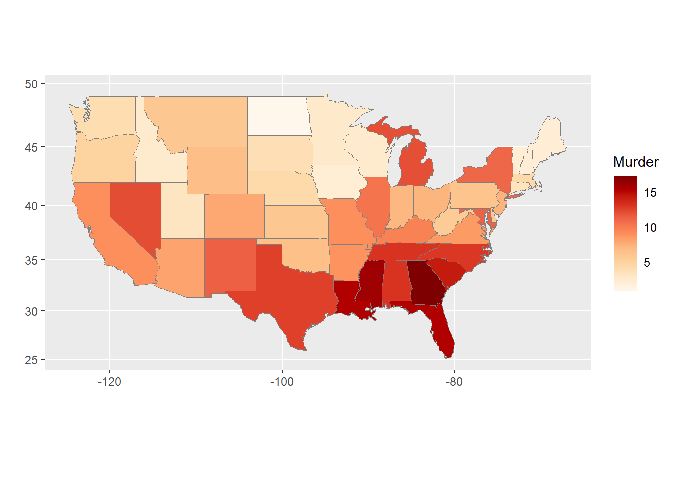
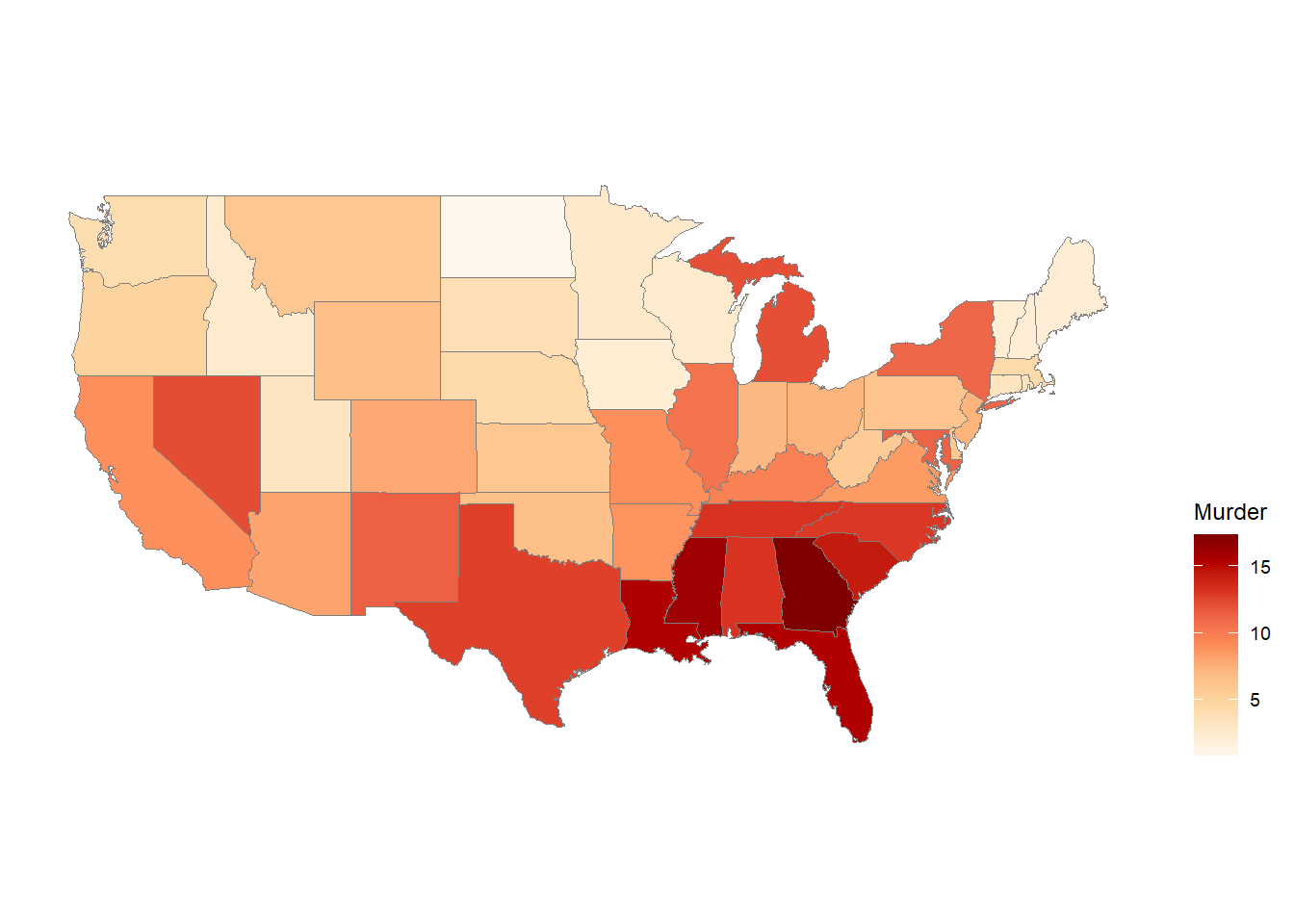
  • Murder: Murder arrests (number of arrests for murder per 100,000 residents).

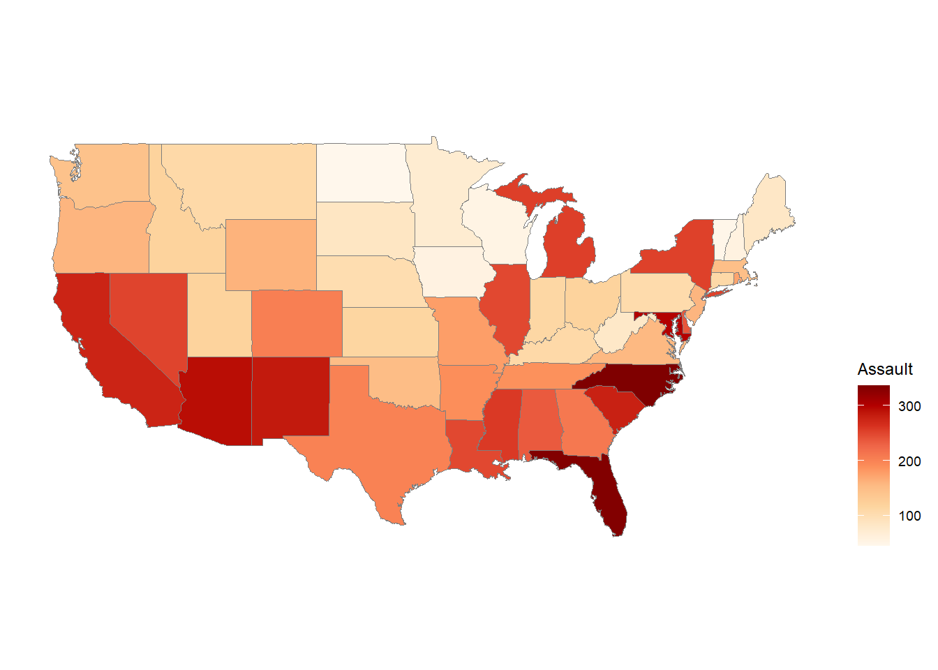
  • Assault: Assault arrests (number of arrests for assault per 100,000 residents).

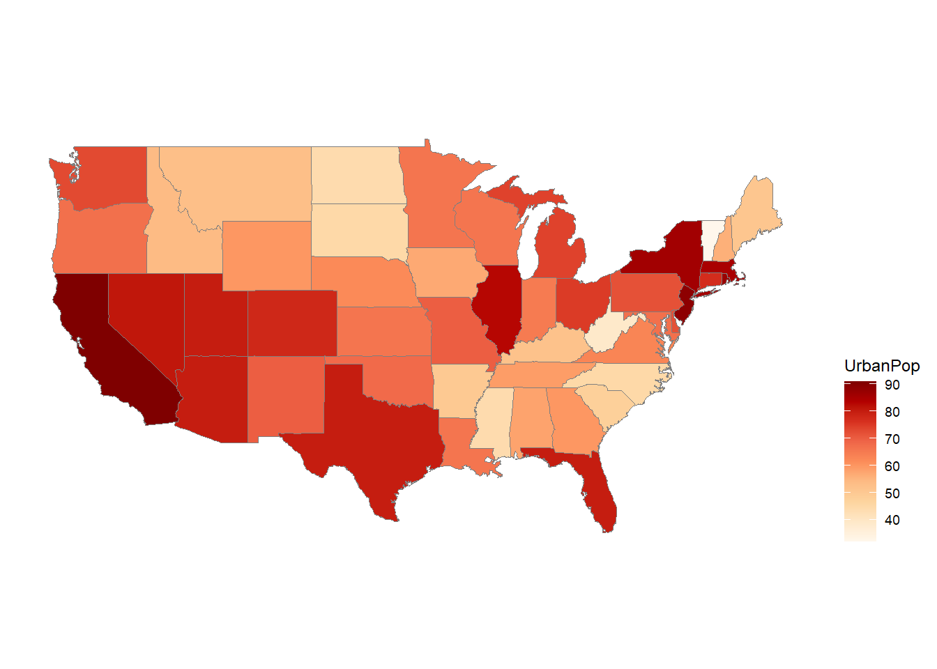
  • UrbanPop: Urban population (percentage of the population living in urban areas).

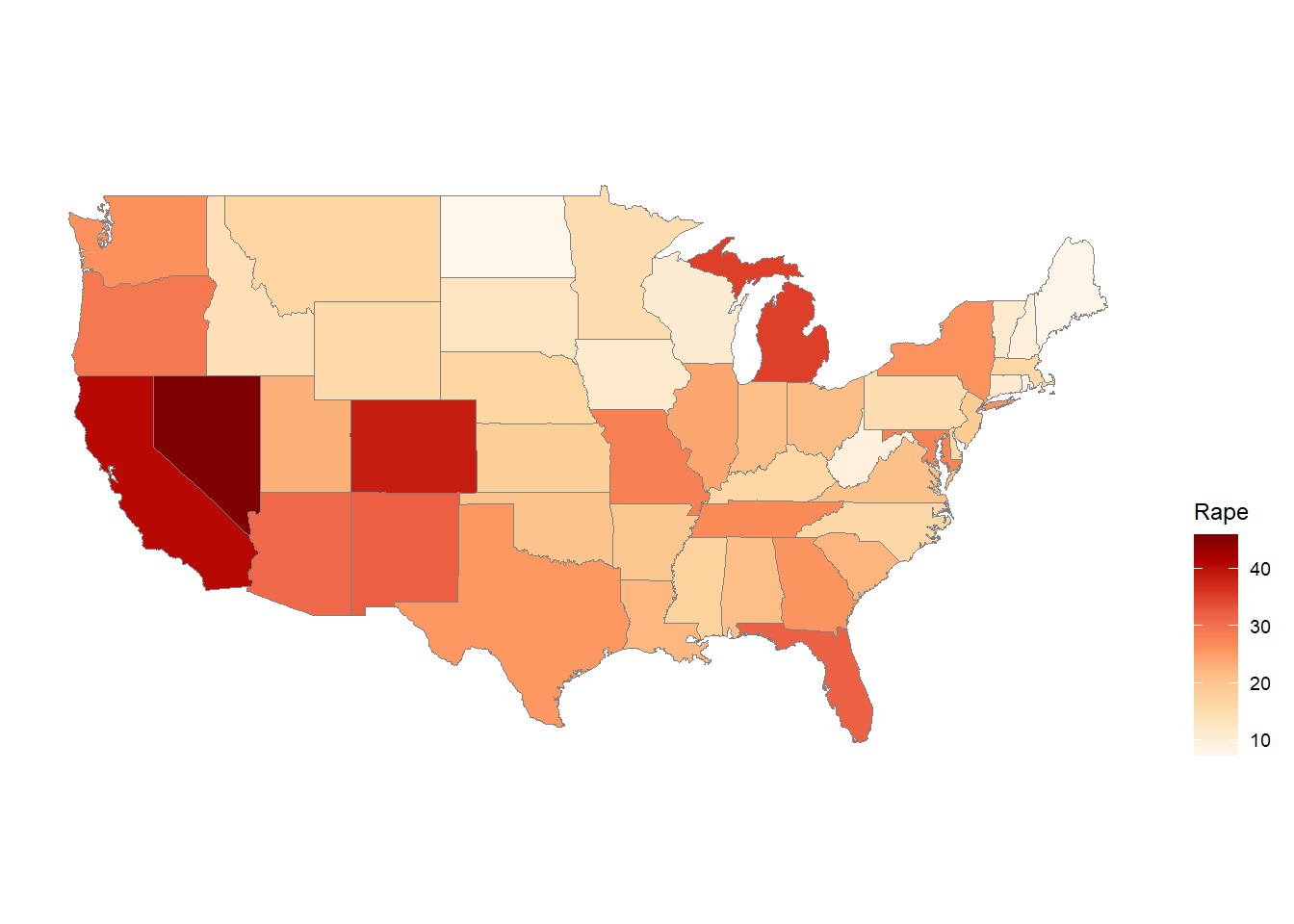
  • Rape: Rape arrests (number of arrests for rape per 100,000 residents).


Visualize the data

See the link for the detail (in Korean)

  • Let’s create a new column for the state name
#change row names to column (variable)
crime <- rownames_to_column(USArrests, var="state") 
head(crime)
       state Murder Assault UrbanPop Rape
1    Alabama   13.2     236       58 21.2
2     Alaska   10.0     263       48 44.5
3    Arizona    8.1     294       80 31.0
4   Arkansas    8.8     190       50 19.5
5 California    9.0     276       91 40.6
6   Colorado    7.9     204       78 38.7
#change the upper letter to lower character in state variable
crime$state <- tolower(crime$state) 
head(crime)
       state Murder Assault UrbanPop Rape
1    alabama   13.2     236       58 21.2
2     alaska   10.0     263       48 44.5
3    arizona    8.1     294       80 31.0
4   arkansas    8.8     190       50 19.5
5 california    9.0     276       91 40.6
6   colorado    7.9     204       78 38.7

The states_map <- map_data("state") code is used to create a dataframe that contains map data for the 50 states in the United States.

The map_data() function is from the ggplot2 package, and it returns a dataframe that contains latitude and longitude coordinates for the boundaries of each state, along with additional information that can be used to plot the map.

The argument to the map_data() function is the name of the region for which to retrieve the map data. In this case, the argument is "state", which indicates that we want map data for the 50 states in the US.

The resulting states_map dataframe contains the following columns:

  • long: A vector of longitudes representing the boundaries of the state.

  • lat: A vector of latitudes representing the boundaries of the state.

  • group: An integer indicating the group to which each point belongs. This is used to group the points together when plotting the map.

  • order: An integer indicating the order in which the points should be plotted.

  • region: A character string indicating the name of the state.

  • subregion: A character string indicating the name of a subregion within the state, if applicable. This is usually NA for the state maps.

states_map <- map_data("state")
head(states_map)
       long      lat group order  region subregion
1 -87.46201 30.38968     1     1 alabama      <NA>
2 -87.48493 30.37249     1     2 alabama      <NA>
3 -87.52503 30.37249     1     3 alabama      <NA>
4 -87.53076 30.33239     1     4 alabama      <NA>
5 -87.57087 30.32665     1     5 alabama      <NA>
6 -87.58806 30.32665     1     6 alabama      <NA>

The code library(ggiraphExtra) loads the ggiraphExtra package, which extends the functionality of the ggplot2 package to allow for interactive graphics in R.

The ggChoropleth() function is from the ggiraphExtra package and is used to create a choropleth map in which each state is colored according to its value of a specified variable.

The first argument to ggChoropleth() is the data frame containing the data to be plotted, which is crime in this case.

The second argument is the aes() function, which is used to map variables in the data frame to visual properties of the plot. The fill aesthetic is used to specify that the color of each state should be determined by the value of the Murder variable in the crime data frame. The map_id aesthetic is used to specify that each state should be identified by its name, which is found in the state variable in the crime data frame.

The third argument is the map argument, which specifies the data frame containing the map data. In this case, the states_map data frame is used, which was created earlier using the map_data() function.

# install.packages("ggiraphExtra")
library(ggiraphExtra)

ggChoropleth(data=crime, aes(fill=Murder, map_id=state), map=states_map)

  • Remove legend and change background color

  • Murder rate by state

library(ggthemes)

Attaching package: 'ggthemes'
The following object is masked from 'package:ggiraphExtra':

    theme_clean
ggChoropleth(data=crime, aes(fill=Murder, map_id=state), map=states_map) + 
  theme_map() + theme(legend.position="right")

  • Urban pop by state
ggChoropleth(data=crime, aes(fill=UrbanPop, map_id=state), map=states_map) + 
  theme_map() + theme(legend.position="right")

  • Assault rate by state
ggChoropleth(data=crime, aes(fill=Assault, map_id=state), map=states_map) + 
  theme_map() + theme(legend.position="right")

  • Rape rate by state
ggChoropleth(data=crime, aes(fill=Rape, map_id=state), map=states_map) + 
  theme_map() + theme(legend.position="right")

Required R packages and functions The standard R function for k-means clustering is kmeans() [stats package], which simplified format is as follow:

kmeans(x, centers, iter.max = 10, nstart = 1)

glimpse(USArrests)
Rows: 50
Columns: 4
$ Murder   <dbl> 13.2, 10.0, 8.1, 8.8, 9.0, 7.9, 3.3, 5.9, 15.4, 17.4, 5.3, 2.…
$ Assault  <int> 236, 263, 294, 190, 276, 204, 110, 238, 335, 211, 46, 120, 24…
$ UrbanPop <int> 58, 48, 80, 50, 91, 78, 77, 72, 80, 60, 83, 54, 83, 65, 57, 6…
$ Rape     <dbl> 21.2, 44.5, 31.0, 19.5, 40.6, 38.7, 11.1, 15.8, 31.9, 25.8, 2…
  • Z-score Standardization for k-means clustering
df <- scale(USArrests) # Scaling the data
head(df)
               Murder   Assault   UrbanPop         Rape
Alabama    1.24256408 0.7828393 -0.5209066 -0.003416473
Alaska     0.50786248 1.1068225 -1.2117642  2.484202941
Arizona    0.07163341 1.4788032  0.9989801  1.042878388
Arkansas   0.23234938 0.2308680 -1.0735927 -0.184916602
California 0.27826823 1.2628144  1.7589234  2.067820292
Colorado   0.02571456 0.3988593  0.8608085  1.864967207
summary(df)
     Murder           Assault           UrbanPop             Rape        
 Min.   :-1.6044   Min.   :-1.5090   Min.   :-2.31714   Min.   :-1.4874  
 1st Qu.:-0.8525   1st Qu.:-0.7411   1st Qu.:-0.76271   1st Qu.:-0.6574  
 Median :-0.1235   Median :-0.1411   Median : 0.03178   Median :-0.1209  
 Mean   : 0.0000   Mean   : 0.0000   Mean   : 0.00000   Mean   : 0.0000  
 3rd Qu.: 0.7949   3rd Qu.: 0.9388   3rd Qu.: 0.84354   3rd Qu.: 0.5277  
 Max.   : 2.2069   Max.   : 1.9948   Max.   : 1.75892   Max.   : 2.6444  

To create a beautiful graph of the clusters generated with the kmeans() function, will use the factoextra package.

# install.packages("factoextra")
library(factoextra)
Welcome! Want to learn more? See two factoextra-related books at https://goo.gl/ve3WBa
  • How many clusters (k) is the best?
g1<-fviz_nbclust(df, kmeans, method = "wss")
g1

g2<-fviz_nbclust(df, kmeans, method = "silhouette")
g2

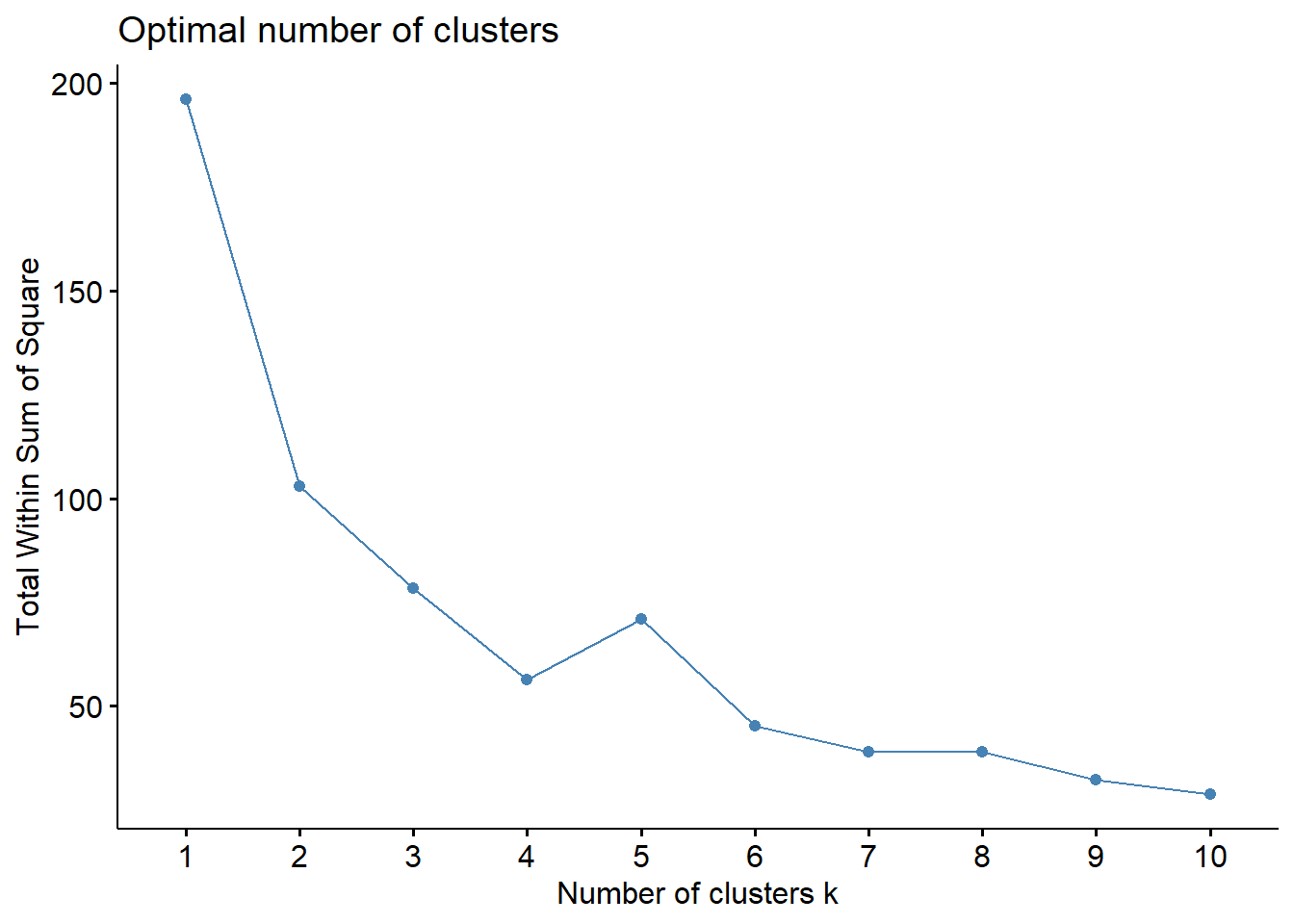
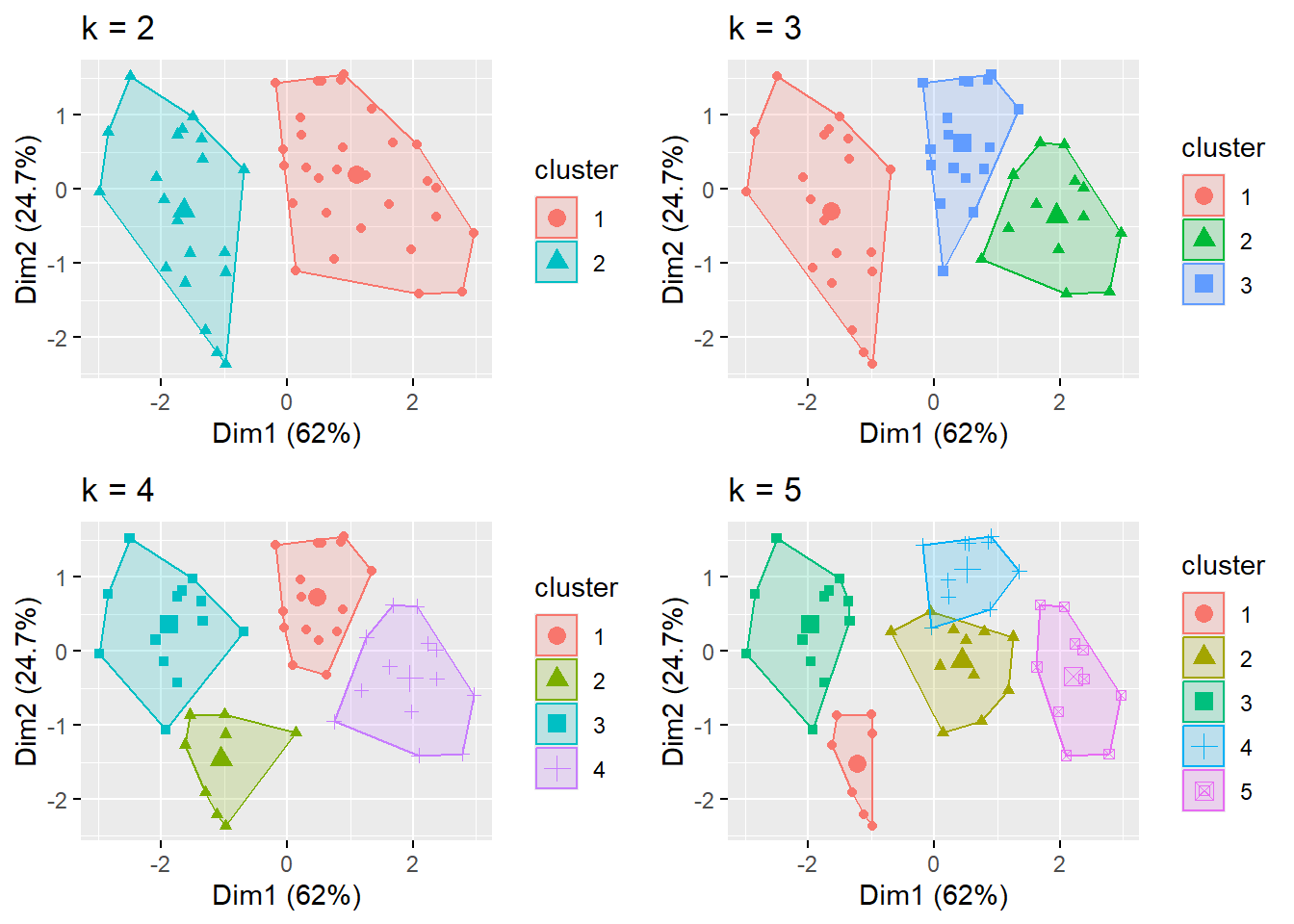
This code uses the fviz_nbclust() function from the factoextra package in R to determine the optimal number of clusters to use in a K-means clustering analysis.

The first argument of fviz_nbclust() is the data frame df that contains the variables to be used in the clustering analysis.

The second argument is the clustering function kmeans that specifies the algorithm to be used for clustering.

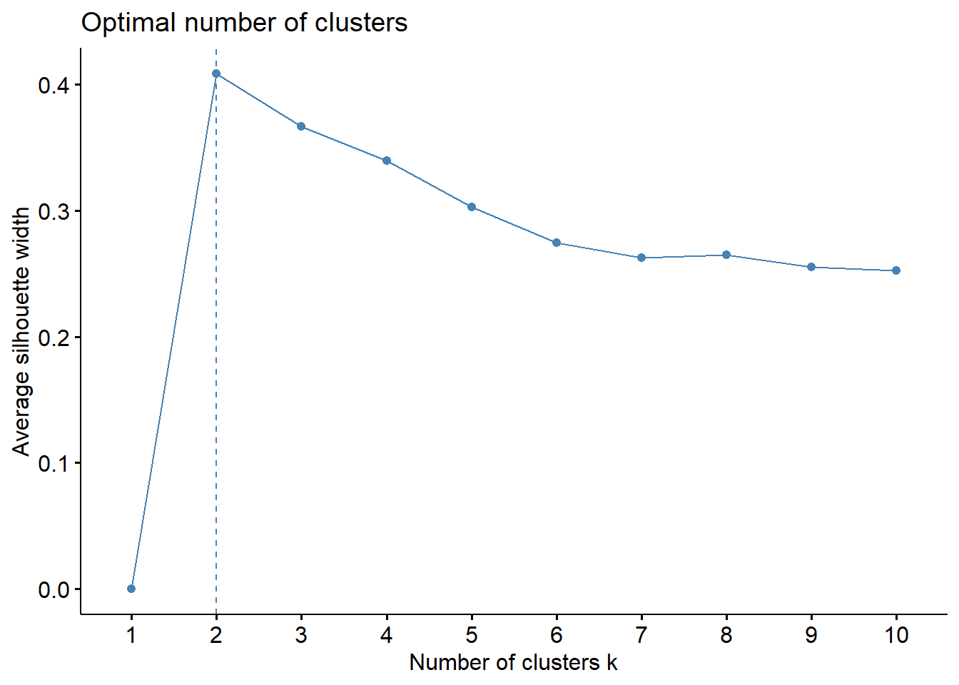
The third argument method specifies the method to be used to determine the optimal number of clusters. In this case, two methods are used:

  • "wss": Within-cluster sum of squares. This method computes the sum of squared distances between each observation and its assigned cluster center, and then adds up these values across all clusters. The goal is to find the number of clusters that minimize the within-cluster sum of squares.

  • "silhouette": Silhouette width. This method computes a silhouette width for each observation, which measures how similar the observation is to its own cluster compared to other clusters. The goal is to find the number of clusters that maximize the average silhouette width across all observations.

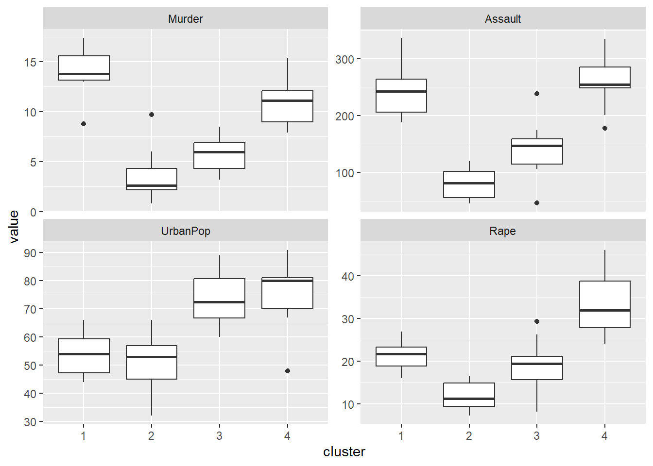
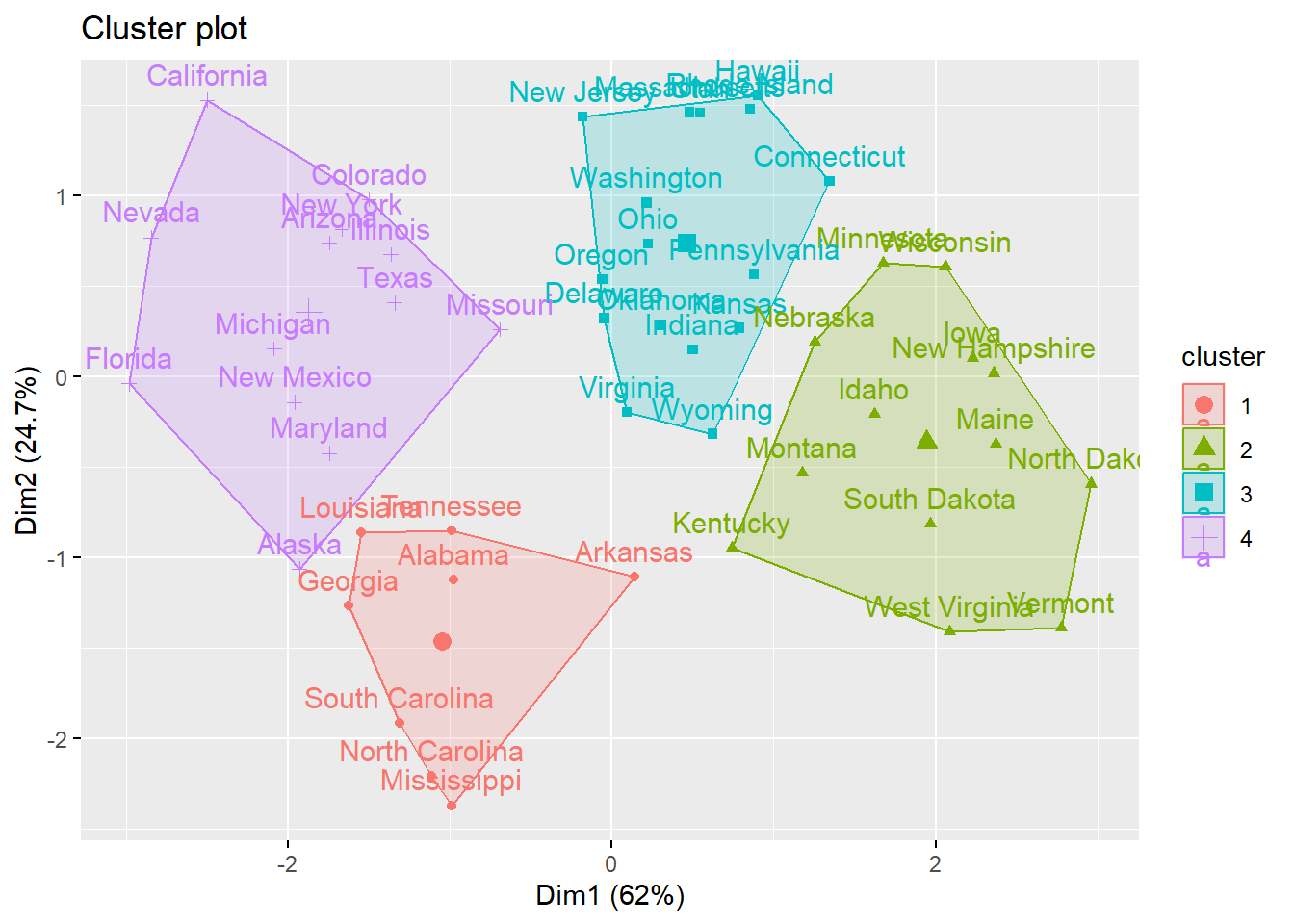
Let’s run unsupervised clustering given k=4

# Compute k-means with k = 4
set.seed(123)
km.res <- kmeans(df, 4, nstart = 25)

As the final result of k-means clustering result is sensitive to the random starting assignments, we specify nstart = 25. This means that R will try 25 different random starting assignments and then select the best results corresponding to the one with the lowest within cluster variation. The default value of nstart in R is one. But, it’s strongly recommended to compute k-means clustering with a large value of nstart such as 25 or 50, in order to have a more stable result.

  • Print the result
# Print the results
print(km.res)
K-means clustering with 4 clusters of sizes 8, 13, 16, 13

Cluster means:
      Murder    Assault   UrbanPop        Rape
1  1.4118898  0.8743346 -0.8145211  0.01927104
2 -0.9615407 -1.1066010 -0.9301069 -0.96676331
3 -0.4894375 -0.3826001  0.5758298 -0.26165379
4  0.6950701  1.0394414  0.7226370  1.27693964

Clustering vector:
       Alabama         Alaska        Arizona       Arkansas     California 
             1              4              4              1              4 
      Colorado    Connecticut       Delaware        Florida        Georgia 
             4              3              3              4              1 
        Hawaii          Idaho       Illinois        Indiana           Iowa 
             3              2              4              3              2 
        Kansas       Kentucky      Louisiana          Maine       Maryland 
             3              2              1              2              4 
 Massachusetts       Michigan      Minnesota    Mississippi       Missouri 
             3              4              2              1              4 
       Montana       Nebraska         Nevada  New Hampshire     New Jersey 
             2              2              4              2              3 
    New Mexico       New York North Carolina   North Dakota           Ohio 
             4              4              1              2              3 
      Oklahoma         Oregon   Pennsylvania   Rhode Island South Carolina 
             3              3              3              3              1 
  South Dakota      Tennessee          Texas           Utah        Vermont 
             2              1              4              3              2 
      Virginia     Washington  West Virginia      Wisconsin        Wyoming 
             3              3              2              2              3 

Within cluster sum of squares by cluster:
[1]  8.316061 11.952463 16.212213 19.922437
 (between_SS / total_SS =  71.2 %)

Available components:

[1] "cluster"      "centers"      "totss"        "withinss"     "tot.withinss"
[6] "betweenss"    "size"         "iter"         "ifault"      

The printed output displays: the cluster means or centers: a matrix, which rows are cluster number (1 to 4) and columns are variables the clustering vector: A vector of integers (from 1:k) indicating the cluster to which each point is allocated

If you want to add the point classifications to the original data, use this:

str(km.res)
List of 9
 $ cluster     : Named int [1:50] 1 4 4 1 4 4 3 3 4 1 ...
  ..- attr(*, "names")= chr [1:50] "Alabama" "Alaska" "Arizona" "Arkansas" ...
 $ centers     : num [1:4, 1:4] 1.412 -0.962 -0.489 0.695 0.874 ...
  ..- attr(*, "dimnames")=List of 2
  .. ..$ : chr [1:4] "1" "2" "3" "4"
  .. ..$ : chr [1:4] "Murder" "Assault" "UrbanPop" "Rape"
 $ totss       : num 196
 $ withinss    : num [1:4] 8.32 11.95 16.21 19.92
 $ tot.withinss: num 56.4
 $ betweenss   : num 140
 $ size        : int [1:4] 8 13 16 13
 $ iter        : int 2
 $ ifault      : int 0
 - attr(*, "class")= chr "kmeans"
km.res$cluster
       Alabama         Alaska        Arizona       Arkansas     California 
             1              4              4              1              4 
      Colorado    Connecticut       Delaware        Florida        Georgia 
             4              3              3              4              1 
        Hawaii          Idaho       Illinois        Indiana           Iowa 
             3              2              4              3              2 
        Kansas       Kentucky      Louisiana          Maine       Maryland 
             3              2              1              2              4 
 Massachusetts       Michigan      Minnesota    Mississippi       Missouri 
             3              4              2              1              4 
       Montana       Nebraska         Nevada  New Hampshire     New Jersey 
             2              2              4              2              3 
    New Mexico       New York North Carolina   North Dakota           Ohio 
             4              4              1              2              3 
      Oklahoma         Oregon   Pennsylvania   Rhode Island South Carolina 
             3              3              3              3              1 
  South Dakota      Tennessee          Texas           Utah        Vermont 
             2              1              4              3              2 
      Virginia     Washington  West Virginia      Wisconsin        Wyoming 
             3              3              2              2              3 
  • Create a new data frame including cluster information
dd <- data.frame(USArrests, cluster = km.res$cluster)
head(dd)
           Murder Assault UrbanPop Rape cluster
Alabama      13.2     236       58 21.2       1
Alaska       10.0     263       48 44.5       4
Arizona       8.1     294       80 31.0       4
Arkansas      8.8     190       50 19.5       1
California    9.0     276       91 40.6       4
Colorado      7.9     204       78 38.7       4
  • Check groups’ characteristics
dd %>% 
  group_by(cluster) %>% 
  summarize_all(mean)
# A tibble: 4 × 5
  cluster Murder Assault UrbanPop  Rape
    <int>  <dbl>   <dbl>    <dbl> <dbl>
1       1  13.9    244.      53.8  21.4
2       2   3.6     78.5     52.1  12.2
3       3   5.66   139.      73.9  18.8
4       4  10.8    257.      76    33.2
  • Cluster number for each of the observations
table(dd$cluster)

 1  2  3  4 
 8 13 16 13 
  • Reshape the dataset to visualize
library(reshape2)

Attaching package: 'reshape2'
The following object is masked from 'package:tidyr':

    smiths
dd %>% 
  melt(id.vars="cluster") %>% 
  mutate(cluster=as.factor(cluster)) %>% 
  head(20)
   cluster variable value
1        1   Murder  13.2
2        4   Murder  10.0
3        4   Murder   8.1
4        1   Murder   8.8
5        4   Murder   9.0
6        4   Murder   7.9
7        3   Murder   3.3
8        3   Murder   5.9
9        4   Murder  15.4
10       1   Murder  17.4
11       3   Murder   5.3
12       2   Murder   2.6
13       4   Murder  10.4
14       3   Murder   7.2
15       2   Murder   2.2
16       3   Murder   6.0
17       2   Murder   9.7
18       1   Murder  15.4
19       2   Murder   2.1
20       4   Murder  11.3
  • Check groups’ characteristics with ggplot
dd %>% 
  melt(id.vars="cluster") %>% 
  mutate(cluster=as.factor(cluster)) %>% 
  ggplot(aes(x=cluster, y=value))+
  geom_boxplot()+
  facet_wrap(~variable, scale="free_y")

  • cluster 1: Rural area with high murder, assault
  • cluster 2: Peaceful rural areas
  • cluster 3: Good city with low crime
  • cluster 4: City Gotham…?

Let’s see clusters are well made

fviz_cluster(km.res, data = df)

Let’s play with different k (number of clusters)

k2 <- kmeans(df, centers = 2, nstart = 25)
k3 <- kmeans(df, centers = 3, nstart = 25)
k4 <- kmeans(df, centers = 4, nstart = 25)
k5 <- kmeans(df, centers = 5, nstart = 25)

# plots to compare
p1 <- fviz_cluster(k2, geom = "point", data = df) + ggtitle("k = 2")
p2 <- fviz_cluster(k3, geom = "point",  data = df) + ggtitle("k = 3")
p3 <- fviz_cluster(k4, geom = "point",  data = df) + ggtitle("k = 4")
p4 <- fviz_cluster(k5, geom = "point",  data = df) + ggtitle("k = 5")

library(gridExtra)

Attaching package: 'gridExtra'
The following object is masked from 'package:dplyr':

    combine
grid.arrange(p1, p2, p3, p4, nrow = 2)