A large number of relatively uncorrelated models (trees) operating as a committee will outperform any of the individual constituent models.
The Random Forest algorithm has become an essential tool in the world of machine learning and data science due to its remarkable performance in solving complex classification and regression problems. The popularity of this algorithm stems from its ability to create a multitude of decision trees, each contributing to the final output, thus providing a robust and accurate model. Let’s explore the ins and outs of the Random Forest algorithm, its benefits, and its applications in various industries.
What is the Random Forest Algorithm?
The Random Forest algorithm is an ensemble learning method that combines multiple decision trees, each trained on different subsets of the dataset. The final prediction is generated by aggregating the results from each tree, typically through a majority vote for classification or averaging for regression problems.
How Does the Random Forest Algorithm Work?
The random forest is a classification algorithm consisting of many decisions trees. It uses bagging and feature randomness when building each individual tree to try to create an uncorrelated forest of trees whose prediction by committee is more accurate than that of any individual tree.
The Random Forest algorithm works through the following steps:
Bootstrapping: Random samples with replacement are drawn from the original dataset, creating several smaller datasets called bootstrap samples.
Decision tree creation: A decision tree is built for each bootstrap sample. During the construction of each tree, a random subset of features is chosen to split the data at each node. This randomness ensures that each tree is diverse and less correlated with others.
Aggregation: Once all the decision trees are built, they are combined to make the final prediction. For classification tasks, this is done by taking the majority vote from all the trees, while for regression tasks, the average prediction is used.
Advantages of the Random Forest Algorithm
The Random Forest algorithm offers several benefits:
High accuracy: By combining multiple decision trees, the algorithm minimizes the risk of overfitting and produces more accurate predictions than a single tree.
Handling missing data: The algorithm can handle missing data efficiently, as it uses information from other trees when making predictions.
Feature importance: The Random Forest algorithm can rank the importance of features, providing valuable insights into which variables contribute the most to the model’s predictive power.
Versatility: The algorithm is applicable to both classification and regression tasks, making it a versatile choice for various problem types.
Real-World Applications of Random Forest
Healthcare: In medical diagnosis, the algorithm can predict diseases based on patient data, improving the accuracy and efficiency of healthcare professionals.
Finance: The algorithm is used in credit scoring, fraud detection, and stock market predictions, enhancing the decision-making process for financial institutions.
Marketing: The algorithm helps in customer segmentation, identifying potential customers, and predicting customer churn, allowing businesses to make informed marketing decisions.
Environment: The Random Forest algorithm is used in remote sensing, climate modeling, and species distribution modeling, assisting researchers and policymakers in environmental conservation and management.
Hands-on practice
First, make sure to install and load the randomForest package:
# Install the package if you haven't already# if (!requireNamespace("randomForest", quietly = TRUE)) {# install.packages("randomForest")# }# Load the packagelibrary(randomForest)
randomForest 4.7-1.1
Type rfNews() to see new features/changes/bug fixes.
Now, let’s create a random forest model using the iris dataset:
Splitting the dataset
# Load the iris datasetdata(iris)# Split the dataset into training (70%) and testing (30%) setsset.seed(42) # Set the seed for reproducibilitysample_size <-floor(0.7*nrow(iris))train_index <-sample(seq_len(nrow(iris)), size = sample_size)train_index
# Create the random forest modelrf_model <-randomForest(Species ~ ., data = iris_train, ntree =500, mtry =2, importance =TRUE)# Print the model summaryprint(rf_model)
Call:
 randomForest(formula = Species ~ ., data = iris_train, ntree = 500,      mtry = 2, importance = TRUE)
               Type of random forest: classification
                     Number of trees: 500
No. of variables tried at each split: 2

        OOB estimate of  error rate: 5.71%
Confusion matrix:
           setosa versicolor virginica class.error
setosa         38          0         0  0.00000000
versicolor      0         33         2  0.05714286
virginica       0          4        28  0.12500000
This code creates a random forest model with 500 trees (ntree = 500) and 2 variables tried at each split (mtry = 2). The importance = TRUE argument calculates variable importance.
Please see the details below.
Call: This is the function call that was used to create the random forest model. It shows the formula used (Species ~ .), the dataset (iris_train), the number of trees (ntree = 500), the number of variables tried at each split (mtry = 2), and whether variable importance was calculated (importance = TRUE).
Type of random forest: This indicates the type of problem the random forest model is built for. In this case, it’s a classification problem since we are predicting the species of iris flowers.
Number of trees: This is the number of decision trees that make up the random forest model. In this case, there are 500 trees.
No. of variables tried at each split: This is the number of variables (features) that are randomly selected at each node for splitting. Here, 2 variables are tried at each split.
OOB estimate of error rate: The Out-of-Bag (OOB) error rate is an estimate of the model’s classification error based on the observations that were not included in the bootstrap sample (i.e., left out) for each tree during the training process. In this case, the OOB error rate is 5.71%, which means that the model misclassified about 5.71% of the samples in the training data.
Confusion matrix: The confusion matrix shows the number of correct and incorrect predictions made by the random forest model for each class in the training data. The diagonal elements represent correct predictions, and the off-diagonal elements represent incorrect predictions. In this case, the model correctly predicted 38 setosa, 33 versicolor, and 28 virginica samples. It misclassified 2 versicolor samples as virginica and 4 virginica samples as versicolor.
class.error: This column displays the error rate for each class. The error rate for setosa is 0% (no misclassifications), 5.71% for versicolor (2 misclassifications), and 12.5% for virginica (4 misclassifications).
In a Random Forest algorithm, hyperparameters are adjustable settings that control the learning process and model’s behavior. Selecting the right hyperparameters is critical to achieving optimal performance. Here, we discuss some common hyperparameters in Random Forest and how to adjust them using the R programming language.
# Train the Random Forest model with custom hyperparametersmodel <-randomForest( Species ~ ., data = iris_train,ntree =100, # n_estimatorsmtry =6, # max_featuresmaxnodes =30, # max_depth (use maxnodes instead)min.node.size =10, # min_samples_splitnodesize =5, # min_samples_leafreplace =TRUE# bootstrap)
Warning in randomForest.default(m, y, ...): invalid mtry: reset to within valid
range
n_estimators: The number of decision trees in the forest. A higher value typically results in better performance but increases computation time.
max_features: The maximum number of features considered at each split in a decision tree. Some common values are ‘auto’, ‘sqrt’, or a float representing a percentage of the total features.
max_depth: The maximum depth of each decision tree. A deeper tree captures more complex patterns but may also lead to overfitting.
min_samples_split: The minimum number of samples required to split an internal node. Higher values reduce overfitting by limiting the depth of the tree.
min_samples_leaf: The minimum number of samples required to be at a leaf node. This parameter prevents the creation of very small leaves, which can help avoid overfitting.
bootstrap: A boolean value indicating whether bootstrap samples are used when building trees. If set to FALSE, the whole dataset is used to build each tree.
To find the best hyperparameters, you can perform a grid search or use other optimization techniques such as random search or Bayesian optimization. The caret package in R can help you with hyperparameter tuning. We will learn this later on.
To make predictions using the model and evaluate its accuracy, use the following code:
# Make predictions using the testing datasetpredictions <-predict(rf_model, iris_test)predictions
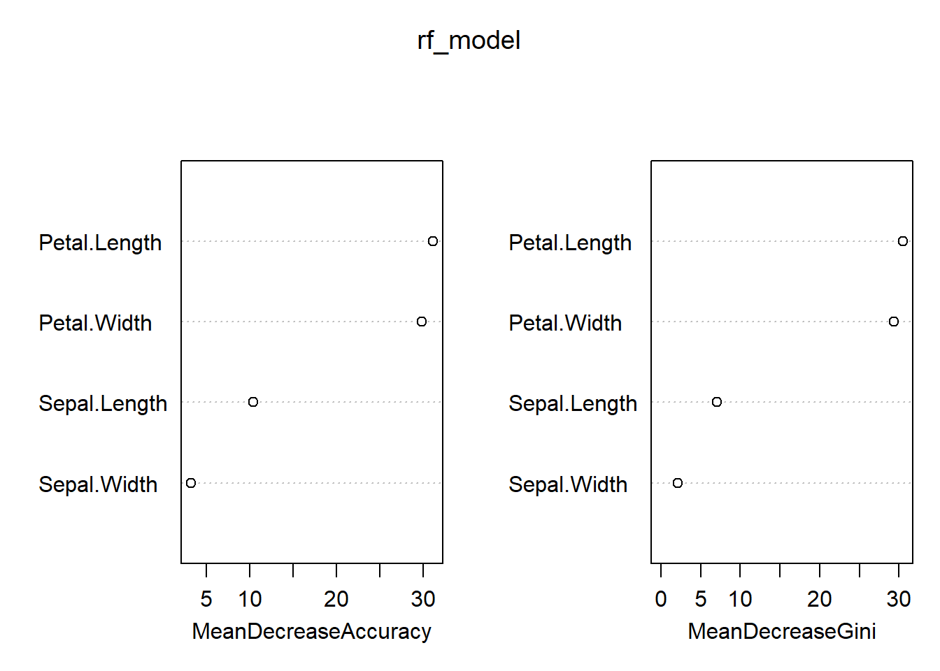
There are two measures of variable importance presented: Mean Decrease in Accuracy and Mean Decrease in Gini Impurity. Both measures provide an indication of how important a given feature is for the model’s performance.
Mean Decrease in Accuracy: This measure calculates the decrease in model accuracy when the values of a specific feature are randomly permuted (keeping all other features the same). A higher value indicates that the feature is more important for the model’s performance. In this case, the order of importance is: Petal.Length (31.14), Petal.Width (29.80), Sepal.Length (10.43), and Sepal.Width (3.21).
Mean Decrease in Gini Impurity: This measure calculates the average decrease in Gini impurity for a specific feature when it is used in trees of the random forest model. The Gini impurity is a measure of how “mixed” the classes are in a given node, with a lower impurity indicating better separation. A higher Mean Decrease in Gini indicates that the feature is more important for the model’s performance. In this case, the order of importance is: Petal.Length (30.52), Petal.Width (29.39), Sepal.Length (7.08), and Sepal.Width (2.12).
Both measures of variable importance agree on the ranking of the features. Petal.Length and Petal.Width are the most important features for predicting the species of iris flowers, while Sepal.Length and Sepal.Width are less important.
Advanced study
The AdaBoost algorithm is a type of ensemble learning algorithm that combines multiple “weak” classifiers to create a “strong” classifier. A weak classifier is one that performs only slightly better than random guessing (i.e., its accuracy is slightly better than 50%). In contrast, a strong classifier is one that performs well on the classification task. There are many similarities with Random Forest but different in the way of giving weights. If you want to know more about the adaboost algorithm then click (here)