Classification

Decision Tree

Weekly design

Pre-class video

• Learning Types

• Supervised learning & Decision Tree

• Pre-class PPT pdf

---

Discussion

Discussion #2

---

Class

---

Why do we need various ML algorithms?

“Each machine learning algorithm serves a specific purpose, much like how each individual serves a unique role in society. There is no one superior ML algorithm, as each is used for a different purpose.”

1. Different types of data and problems: Different ML algorithms are suited to different types of data and problems. For example, linear regression is well-suited for continuous numerical data, while decision trees are well-suited for categorical data. Similarly, some algorithms are better suited for classification problems (predicting a categorical outcome), while others are better suited for regression problems (predicting a continuous outcome).

2. Performance trade-offs: Different ML algorithms can have different trade-offs in terms of performance and interpretability. For example, some algorithms, like k-nearest neighbors, are simple to understand and interpret, but may not perform as well as more complex algorithms like neural networks. On the other hand, some algorithms, like deep learning, can achieve very high performance, but may be more difficult to interpret.

3. Model assumptions: Different ML algorithms make different assumptions about the relationship between the predictors and the outcome. For example, linear regression assumes a linear relationship, while decision trees do not make this assumption. Selecting the appropriate algorithm depends on the nature of the problem and the data, as well as the goals of the analysis.

4. Computational resources: Some ML algorithms are more computationally intensive than others, and may require more resources (such as memory and processing power) to fit and use. In some cases, a more complex algorithm may be necessary to achieve the desired level of performance, but in other cases, a simpler algorithm may be sufficient.

5. Model interpretability: Some ML algorithms are more interpretable than others, which can be important in certain applications. For example, in medical applications, it may be important to understand why a model is making a certain prediction, while in other applications, it may be more important to simply achieve high accuracy.

The choice of ML algorithm depends on the data, the problem, and the goals of the analysis, and it is important to consider these factors when selecting an algorithm.

Decision Tree

Generates a set of rules that allow for accurate predictions using one explanatory variable at a time, resulting in a structure similar to an inverted tree: decision tree

한번에 하나씩의 설명 변수를 사용하여 정확한 예측이 가능한 규칙들의 집합을 생성.

Terminologies

1. Node: A point in the decision tree where a decision or split is made.

2. Parent node: A node that has other nodes connected to it, called child nodes.

3. Child node: A node that is connected to a parent node and splits off in a different direction in the tree.

4. Split criterion: The criterion used to determine the split at each node in the decision tree. This can be based on various measures such as information gain, Gini impurity, or chi-squared statistic.

5. Root node: The top node in the decision tree that represents the entire dataset.

6. Leaf node: A node in the decision tree that represents a final prediction or classification, as it does not have any child nodes connected to it.

Then, “Why is it called a ‘decision’ tree?”

• This is because it presents results in the form of easily understandable rules,

• reduces the need for pre-processing data such as normalization or imputation,

• and considers both numeric and categorical variables as its independent variables (features).

Essential ideas of decision tree

• Recursive Partitioning: The process of dividing the input variable space into two parts, with the goal of increasing the purity of each area after separation rather than before separation

• Pruning the Tree: The process of consolidating areas that have been separated into overly detailed regions in order to prevent overfitting.”

Impurity index 1: Gini index

\[ I(A)=1-\sum_{k = 1}^{c} p_k^2 \]

• \(I(A)\) is Gini index of A area in which there is c number of classes

• \(P_k\) is number of observations in k class

\[ I(A)=1-\sum_{k = 1}^{c} p_k^2 =1-(\frac{6}{16})^2-(\frac{10}{16})^2 = 0.4688 \]

• \(I(A)\) is 0 when there are only one category in area c

• \(I(A)\) is 0.5 when there are half of one and half of another category in area c

Gini index when there are two or more areas

\[ I(A)=\sum_{i = 1}^{d} (R_i(1-\sum_{k = 1}^{c} p_{ik}^2)) \]

• After splitting the area A, \(I(A)\) is Gini Index for two or more areas

• \(R_i\) is a ratio of i area in A

\[ I(A)= \frac{8}{16} \times (1-(\frac{7}{8})^2 -(\frac{1}{8})^2)+ \frac{8}{16} \times (1-(\frac{3}{8})^2 -(\frac{5}{8})^2)=0.3438 \]

• After splitting, the information gain is \(0.4668 - 0.3438=0.1250\)

Impurity index 2: Deviance

\[ D_i = -2 \sum_{k}n_{ik} log(P_{ik}) \]

• \(i\) is node index

• \(k\) is class index

• \(P_{ik}\) is a probability of class k in node i

\[ D_i = -2 \times (10 \times log (\frac{10}{16}) + 6 \times (\frac{6}{16}))=21.17 \]

\[ D_1 = -2 \times (7 \times log (\frac{7}{8}) + 1 \times log(\frac{1}{8}))=6.03 \]

\[ D_2 = -2 \times (3 \times log (\frac{3}{8}) + 5 \times log(\frac{5}{8}))=10.59 \]

\[ D_1 + D_2 = 16.62 \]

• After splitting, the information gain is \(21.17 - 16.62=4.55\)

Over-fitting issue

• Over-fitting is a common issue in machine learning algorithms, including decision trees. It occurs when a model learns the training data too well and captures not only the underlying patterns but also the noise present in the data. As a result, the model becomes too complex and performs poorly on new, unseen data, even though it may have high accuracy on the training data.

• In the context of decision trees, over-fitting can occur when the tree becomes too deep, with many levels and branches. A deep tree may split the training data into very specific and detailed regions, resulting in a model that is too tailored to the training data and not generalizable to new data.

• To address over-fitting in decision trees, several techniques can be employed:

1. Pruning: This involves trimming the tree by removing branches that do not significantly improve the model’s performance. Pruning can be done in a top-down manner (pre-pruning), where the tree is stopped from growing further once a certain depth or node count is reached, or in a bottom-up manner (post-pruning), where the tree is fully grown and then branches are removed based on certain criteria.

2. Limiting tree depth: By setting a maximum depth for the tree, the algorithm is forced to make fewer splits and create a simpler model, reducing the likelihood of over-fitting.

3. Using minimum node size: Setting a minimum number of samples required to create a split or leaf node can prevent the tree from making splits that are too specific to the training data.

4. Cross-validation: This technique involves splitting the data into multiple training and validation sets and averaging the model’s performance across these sets. Cross-validation can help in choosing the optimal tree depth and other hyper-parameters that lead to the best generalization performance.

Pruning

A technique used to reduce over-fitting in decision tree models by removing branches that do not significantly improve model performance.

• Goal: To simplify the tree, improving generalizability and reducing complexity, while maintaining prediction accuracy.

• Two main types of pruning:

  1. Pre-pruning (Top-down): Stops tree growth once certain criteria are met, such as maximum depth or minimum node size.

  2. Post-pruning (Bottom-up): Allows the tree to fully grow, then iteratively removes branches based on specific criteria, such as error rate or information gain.

• Criteria for pruning: Can be based on various measures, such as error rate, information gain, or Gini impurity, and the cost of complexity (CC)

• Cross-validation: Often used in conjunction with pruning to determine the optimal level of pruning, by comparing model performance on multiple training and validation sets.

• Benefits: Pruning can lead to better generalization performance, reduced over-fitting, and more interpretable models.

Cost of complexity

\[ CC(T)=Err(T)+\alpha L(T) \]

• \(CC(T)\) is cost of complexity

• \(Err(T)\) is error rate of Tree with test dataset

• \(L(T)\) is the number of last nodes of Tree

• \(\alpha\) is weight of combining Err(T) and L(T): depends on researcher’s decision.

Cost of complexity Example #1

• Tree 1: Err(T) = 10%

• Tree 2: Err(T) = 15%

• Choose Tree A is better as the same number of last nodes

Cost of complexity Example #2

• Tree A: Err(T) = 15%

• Tree B: Err(T) = 15%

• Choose Tree A is better as the same Err(T) but low number of last nodes

Practice with data

head(iris, 10)

   Sepal.Length Sepal.Width Petal.Length Petal.Width Species
1           5.1         3.5          1.4         0.2  setosa
2           4.9         3.0          1.4         0.2  setosa
3           4.7         3.2          1.3         0.2  setosa
4           4.6         3.1          1.5         0.2  setosa
5           5.0         3.6          1.4         0.2  setosa
6           5.4         3.9          1.7         0.4  setosa
7           4.6         3.4          1.4         0.3  setosa
8           5.0         3.4          1.5         0.2  setosa
9           4.4         2.9          1.4         0.2  setosa
10          4.9         3.1          1.5         0.1  setosa

Using ‘rpart’ to train the model with the ‘iris’ dataset

• The target (response) variable should be ‘factor’ in R
• Or, use rpart(…, method=‘class’) option
• Otherwise, rpart do regression instead of classification
• Then, let’s train the model with the data ‘iris’

library(rpart)
r = rpart(Species ~ ., data = iris)
print(r)

n= 150 

node), split, n, loss, yval, (yprob)
      * denotes terminal node

1) root 150 100 setosa (0.33333333 0.33333333 0.33333333)  
  2) Petal.Length< 2.45 50   0 setosa (1.00000000 0.00000000 0.00000000) *
  3) Petal.Length>=2.45 100  50 versicolor (0.00000000 0.50000000 0.50000000)  
    6) Petal.Width< 1.75 54   5 versicolor (0.00000000 0.90740741 0.09259259) *
    7) Petal.Width>=1.75 46   1 virginica (0.00000000 0.02173913 0.97826087) *

• Tree visualization

par(mfrow = c(1,1), xpd = NA)
plot(r)
text(r, use.n = T)

• The question of the root node (node 0): [Petal.Length<2.45?]
  • Yes of 50 to the left,
  • No of 100 to the right among 150 sample
  • 50 on the left all belong to ‘setosa’ so STOP 🡪 Make a leaf and record setosa(50/0/0)
• The child node on the right side of the root: [Petal.Width<1.75?]
  • Yes of 54 to the left,
  • and No of 46 to the right among the 100
• On the left 54, there are 49 versicolor and 5 virginica 🡪 To avoid overfitting the algorithm STOP and record versicolor(0/49/5).
• On the right 46, there are 1 versicolor and 45 virginica 🡪 To avoid overfitting the algorithm STOP and record virginica(0/1/45).

Prediction

• Use the function ‘prediction’
• type=‘class’ option prints the class (the default is type=‘prob’ which prints probability of each class)

p = predict(r, iris, type = 'class')
head(p, 10)

     1      2      3      4      5      6      7      8      9     10 
setosa setosa setosa setosa setosa setosa setosa setosa setosa setosa 
Levels: setosa versicolor virginica

• Confusion matrix

  • Show the correct and the wrong classifications in detail
  • See below for example, among 50 versicolor, 49 are correct but one is wrong to virginica

  table(p, iris$Species)

  
  p            setosa versicolor virginica
    setosa         50          0         0
    versicolor      0         49         5
    virginica       0          1        45

  
  

New data is from train data but a little bit of change is given.

newd = data.frame(Sepal.Length = c(5.11, 7.01, 6.32),
                  Sepal.Width = c(3.51, 3.2, 3.31),
                  Petal.Length = c(1.4, 4.71, 6.02),
                  Petal.Width = c(0.19, 1.4, 2.49))
newd

  Sepal.Length Sepal.Width Petal.Length Petal.Width
1         5.11        3.51         1.40        0.19
2         7.01        3.20         4.71        1.40
3         6.32        3.31         6.02        2.49

predict(r, newdata = newd)

  setosa versicolor  virginica
1      1 0.00000000 0.00000000
2      0 0.90740741 0.09259259
3      0 0.02173913 0.97826087

Let’s read the result with the ‘function ’summary’

summary(r)

Call:
rpart(formula = Species ~ ., data = iris)
  n= 150 

    CP nsplit rel error xerror       xstd
1 0.50      0      1.00   1.17 0.05073460
2 0.44      1      0.50   0.64 0.06057502
3 0.01      2      0.06   0.10 0.03055050

Variable importance
 Petal.Width Petal.Length Sepal.Length  Sepal.Width 
          34           31           21           14 

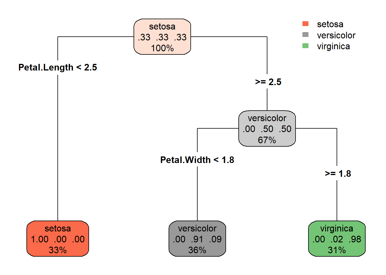
Node number 1: 150 observations,    complexity param=0.5
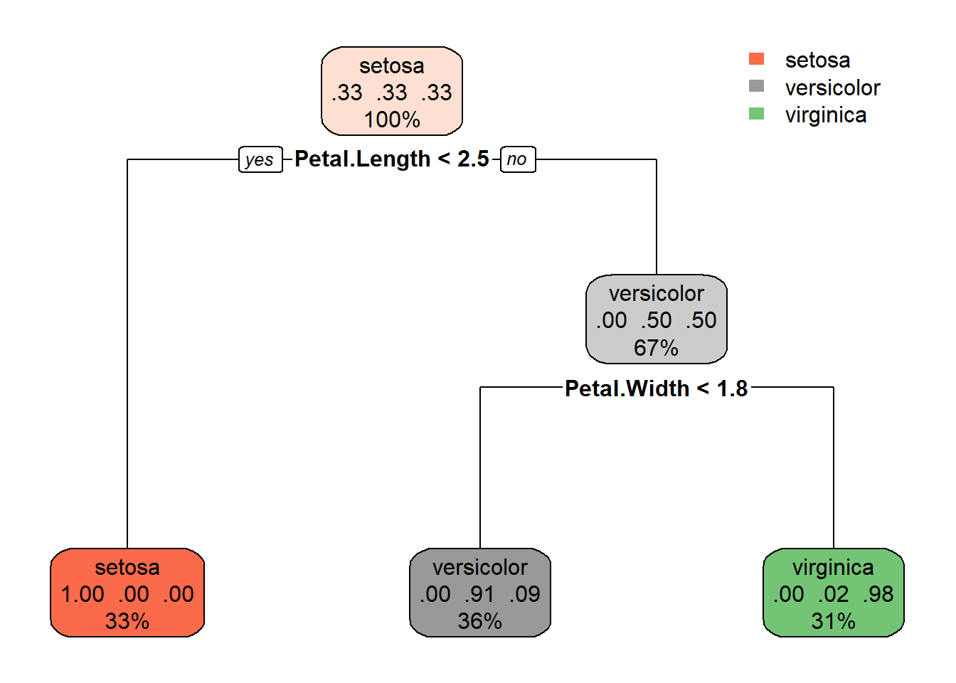
  predicted class=setosa      expected loss=0.6666667  P(node) =1
    class counts:    50    50    50
   probabilities: 0.333 0.333 0.333 
  left son=2 (50 obs) right son=3 (100 obs)
  Primary splits:
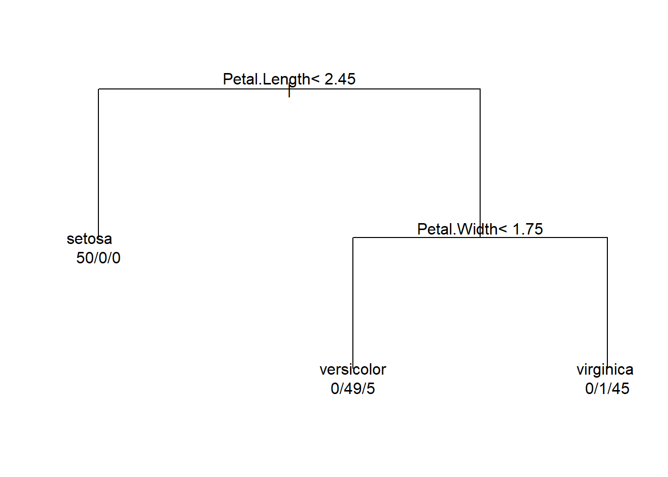
      Petal.Length < 2.45 to the left,  improve=50.00000, (0 missing)
      Petal.Width  < 0.8  to the left,  improve=50.00000, (0 missing)
      Sepal.Length < 5.45 to the left,  improve=34.16405, (0 missing)
      Sepal.Width  < 3.35 to the right, improve=19.03851, (0 missing)
  Surrogate splits:
      Petal.Width  < 0.8  to the left,  agree=1.000, adj=1.00, (0 split)
      Sepal.Length < 5.45 to the left,  agree=0.920, adj=0.76, (0 split)
      Sepal.Width  < 3.35 to the right, agree=0.833, adj=0.50, (0 split)

Node number 2: 50 observations
  predicted class=setosa      expected loss=0  P(node) =0.3333333
    class counts:    50     0     0
   probabilities: 1.000 0.000 0.000 

Node number 3: 100 observations,    complexity param=0.44
  predicted class=versicolor  expected loss=0.5  P(node) =0.6666667
    class counts:     0    50    50
   probabilities: 0.000 0.500 0.500 
  left son=6 (54 obs) right son=7 (46 obs)
  Primary splits:
      Petal.Width  < 1.75 to the left,  improve=38.969400, (0 missing)
      Petal.Length < 4.75 to the left,  improve=37.353540, (0 missing)
      Sepal.Length < 6.15 to the left,  improve=10.686870, (0 missing)
      Sepal.Width  < 2.45 to the left,  improve= 3.555556, (0 missing)
  Surrogate splits:
      Petal.Length < 4.75 to the left,  agree=0.91, adj=0.804, (0 split)
      Sepal.Length < 6.15 to the left,  agree=0.73, adj=0.413, (0 split)
      Sepal.Width  < 2.95 to the left,  agree=0.67, adj=0.283, (0 split)

Node number 6: 54 observations
  predicted class=versicolor  expected loss=0.09259259  P(node) =0.36
    class counts:     0    49     5
   probabilities: 0.000 0.907 0.093 

Node number 7: 46 observations
  predicted class=virginica   expected loss=0.02173913  P(node) =0.3066667
    class counts:     0     1    45
   probabilities: 0.000 0.022 0.978 

• Variable importance shows the order of the explainable (independent) variables which contributes to predicting Y
• When the model is trained, it chooses the features that are important at the same time
• That’s why the first visualization tree used only two variables: Petal.Width and Length

The effective visualization helps to read the results of decision tree

library(rpart.plot)
rpart.plot(r)

You can change a style of the graph

rpart.plot(r, type = 4)

Pros & Cons of DT

• Con: the performance is not that good

• Pros

  • Easy interpretability
    (예를 들어, “꽃받침 길이가 2.54보다 크고, 꽃받침 너비가 1.75보다 작아 versicolor로 분류”했다는 해석을 내놓을 수 있음)

  • Fast prediction (몇 번의 비교 연산으로 분류)

  • Ensemble techniques make DT the great again (e.g. Random Forest)

  • DT accepts categorical variables well (e.g. gender, pclass)