Data Exploration (1)

Loop & Function

Weekly design


Pre-class video


Loop


x = 5
if(x %% 2 ==0) {
   print('x is an even number') # Performed when the conditional expression is true
} else {
   print('x is odd') # Performed when the conditional expression is false
}
[1] "x is odd"
x = 8
if(x>0) {
   print('x is a positive value.') # Print if x is greater than 0
} else if(x<0) {
   print('x is a negative value.') # Prints if the above condition is not satisfied and x is less than 0
} else {
   print('x is zero.') # Prints if all of the above conditions are not met
}
[1] "x is a positive value."
x = c(-5:5)
options(digits = 3) # Set the number of significant digits to 3 when expressing numbers
sqrt(x)
Warning in sqrt(x): NaNs produced
 [1]  NaN  NaN  NaN  NaN  NaN 0.00 1.00 1.41 1.73 2.00 2.24
sqrt(ifelse(x>=0, x, NA)) # Display negative numbers as NA to prevent NaN from occurring
 [1]   NA   NA   NA   NA   NA 0.00 1.00 1.41 1.73 2.00 2.24
students = read.csv("data/students2.csv", fileEncoding = "CP949", encoding = "UTF-8")
students # Data contains values over 100 and negative values.
    name korean english math
1 강서준    100      90  100
2 김도형     90     120   80
3 박정원     90      95   90
4 이상훈    100      85 -100
5 최건우     85     100  100
students[, 2] = ifelse(students[, 2]>= 0 & students[, 2]<= 100,
                        students[, 2], NA)
students[, 3] = ifelse(students[, 3]>= 0 & students[, 3]<= 100,
                        students[, 3], NA)
students[, 4] = ifelse(students[, 4]>= 0 & students[, 4]<= 100,
                        students[, 4], NA)


students 
    name korean english math
1 강서준    100      90  100
2 김도형     90      NA   80
3 박정원     90      95   90
4 이상훈    100      85   NA
5 최건우     85     100  100
# ifelse statement, values other than 0 to 100 among the values in columns 2 to 4 are treated as NA.


# Increment numbers from 1 to 10 using the repeat statement
i = 1 # starting value of i is 1
repeat {
   if(i>10) { # Break repetition if i exceeds 10
     break
   } else {
     print(i)
     i = i+1 # Increment i by 1.
   }
}
[1] 1
[1] 2
[1] 3
[1] 4
[1] 5
[1] 6
[1] 7
[1] 8
[1] 9
[1] 10
# Increment numbers from 1 to 10 using while statement
i = 1 # The starting value of i is 1.
while(i < 10){ # repeat as long as i is less than 10
   print(i)
   i = i+1 # Increment i by 1.
}
[1] 1
[1] 2
[1] 3
[1] 4
[1] 5
[1] 6
[1] 7
[1] 8
[1] 9
# Create the second column of the multiplication table using the while statement
i = 1
while(i<10) {
   print(paste(2, "X", i, "=", 2*i))
   i = i+1
}
[1] "2 X 1 = 2"
[1] "2 X 2 = 4"
[1] "2 X 3 = 6"
[1] "2 X 4 = 8"
[1] "2 X 5 = 10"
[1] "2 X 6 = 12"
[1] "2 X 7 = 14"
[1] "2 X 8 = 16"
[1] "2 X 9 = 18"
# Incrementing numbers from 1 to 10 using the for statement
for(i in 1:10) {
   print(i)
}
[1] 1
[1] 2
[1] 3
[1] 4
[1] 5
[1] 6
[1] 7
[1] 8
[1] 9
[1] 10
# Create the second column of the multiplication table using the for statement
for(i in 1:9) {
   print(paste(2, "X", i, "=", 2*i))
}
[1] "2 X 1 = 2"
[1] "2 X 2 = 4"
[1] "2 X 3 = 6"
[1] "2 X 4 = 8"
[1] "2 X 5 = 10"
[1] "2 X 6 = 12"
[1] "2 X 7 = 14"
[1] "2 X 8 = 16"
[1] "2 X 9 = 18"
# Create multiplication table columns 2 to 9 using the for statement
for(i in 2:9) {
   for(j in 1:9) {
     print(paste(i, "X", j, "=", i*j))
   }
}
[1] "2 X 1 = 2"
[1] "2 X 2 = 4"
[1] "2 X 3 = 6"
[1] "2 X 4 = 8"
[1] "2 X 5 = 10"
[1] "2 X 6 = 12"
[1] "2 X 7 = 14"
[1] "2 X 8 = 16"
[1] "2 X 9 = 18"
[1] "3 X 1 = 3"
[1] "3 X 2 = 6"
[1] "3 X 3 = 9"
[1] "3 X 4 = 12"
[1] "3 X 5 = 15"
[1] "3 X 6 = 18"
[1] "3 X 7 = 21"
[1] "3 X 8 = 24"
[1] "3 X 9 = 27"
[1] "4 X 1 = 4"
[1] "4 X 2 = 8"
[1] "4 X 3 = 12"
[1] "4 X 4 = 16"
[1] "4 X 5 = 20"
[1] "4 X 6 = 24"
[1] "4 X 7 = 28"
[1] "4 X 8 = 32"
[1] "4 X 9 = 36"
[1] "5 X 1 = 5"
[1] "5 X 2 = 10"
[1] "5 X 3 = 15"
[1] "5 X 4 = 20"
[1] "5 X 5 = 25"
[1] "5 X 6 = 30"
[1] "5 X 7 = 35"
[1] "5 X 8 = 40"
[1] "5 X 9 = 45"
[1] "6 X 1 = 6"
[1] "6 X 2 = 12"
[1] "6 X 3 = 18"
[1] "6 X 4 = 24"
[1] "6 X 5 = 30"
[1] "6 X 6 = 36"
[1] "6 X 7 = 42"
[1] "6 X 8 = 48"
[1] "6 X 9 = 54"
[1] "7 X 1 = 7"
[1] "7 X 2 = 14"
[1] "7 X 3 = 21"
[1] "7 X 4 = 28"
[1] "7 X 5 = 35"
[1] "7 X 6 = 42"
[1] "7 X 7 = 49"
[1] "7 X 8 = 56"
[1] "7 X 9 = 63"
[1] "8 X 1 = 8"
[1] "8 X 2 = 16"
[1] "8 X 3 = 24"
[1] "8 X 4 = 32"
[1] "8 X 5 = 40"
[1] "8 X 6 = 48"
[1] "8 X 7 = 56"
[1] "8 X 8 = 64"
[1] "8 X 9 = 72"
[1] "9 X 1 = 9"
[1] "9 X 2 = 18"
[1] "9 X 3 = 27"
[1] "9 X 4 = 36"
[1] "9 X 5 = 45"
[1] "9 X 6 = 54"
[1] "9 X 7 = 63"
[1] "9 X 8 = 72"
[1] "9 X 9 = 81"
# Print only even numbers from 1 to 10
for(i in 1:10) {
   if(i%%2 == 0) {
     print(i)
   }
}
[1] 2
[1] 4
[1] 6
[1] 8
[1] 10
# Print decimal numbers from 1 to 10
for(i in 1:10) {
   check = 0
   for(j in 1:i) {
     if(i%%j ==0) {
       check = check+1
     }
   }
   if(check ==2) {
     print(i)
   }
}
[1] 2
[1] 3
[1] 5
[1] 7
# data contains values over 100 and negative values
students
    name korean english math
1 강서준    100      90  100
2 김도형     90      NA   80
3 박정원     90      95   90
4 이상훈    100      85   NA
5 최건우     85     100  100
for(i in 2:4) {
   students[, i] = ifelse(students[, i]>= 0 & students[, i]<= 100,
                          students[, i], NA)
}


students
    name korean english math
1 강서준    100      90  100
2 김도형     90      NA   80
3 박정원     90      95   90
4 이상훈    100      85   NA
5 최건우     85     100  100

Functions & Others


# 03 User-defined function: Bundle the desired function #
x=5
fa = 1 # Variable to store the factorial value
while(x>1) { # loop while x is greater than 1
  
   fa = fa*x # Multiply the value of x by fa and store it back in fa
   x = x-1 # Decrease x value by 1
   x
}
fa
[1] 120
fact = function(x) { # The name of the function is fact, the input is x
   fa = 1 # Variable to store the factorial value
   while(x>1) { # loop while x is greater than 1
     fa = fa*x # Multiply the value of x by fa and store it back in fa
     x = x-1 # Decrease x value by 1
   }
   return(fa) # returns the final calculated fa
}
fact(5) # Prints the result of calculating 5!
[1] 120
my.is.na<-function(x) { # Create a my.is.na function that combines the table(is.na()) functions into one
   table(is.na(x))
}

my.is.na(airquality) # This result is the same as table(is.na(airquality)).

FALSE  TRUE 
  874    44 
table(is.na(airquality))

FALSE  TRUE 
  874    44 
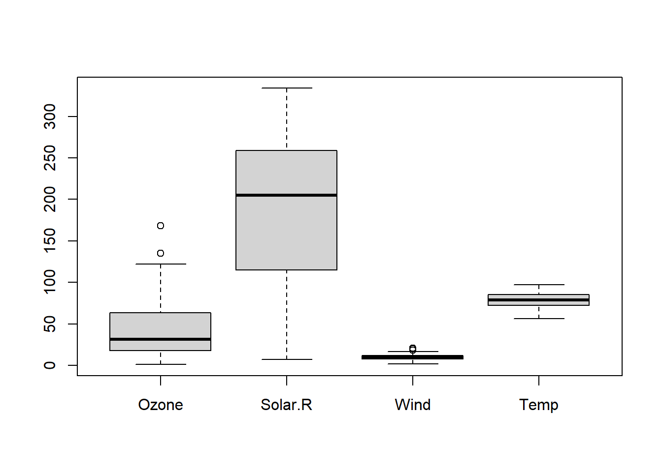
# 04 Data Cleaning Example 1: Missing Value Handling #

# Handling missing values using the is.na function
str(airquality) # Examine the structure of airquality data.
'data.frame':   153 obs. of  6 variables:
 $ Ozone  : int  41 36 12 18 NA 28 23 19 8 NA ...
 $ Solar.R: int  190 118 149 313 NA NA 299 99 19 194 ...
 $ Wind   : num  7.4 8 12.6 11.5 14.3 14.9 8.6 13.8 20.1 8.6 ...
 $ Temp   : int  67 72 74 62 56 66 65 59 61 69 ...
 $ Month  : int  5 5 5 5 5 5 5 5 5 5 ...
 $ Day    : int  1 2 3 4 5 6 7 8 9 10 ...
# NA in airquality data is indicated as TRUE, otherwise it is indicated as FALSE. There is a lot of data, so it is selected using the head function.
head(airquality)
  Ozone Solar.R Wind Temp Month Day
1    41     190  7.4   67     5   1
2    36     118  8.0   72     5   2
3    12     149 12.6   74     5   3
4    18     313 11.5   62     5   4
5    NA      NA 14.3   56     5   5
6    28      NA 14.9   66     5   6
head(is.na(airquality))
     Ozone Solar.R  Wind  Temp Month   Day
[1,] FALSE   FALSE FALSE FALSE FALSE FALSE
[2,] FALSE   FALSE FALSE FALSE FALSE FALSE
[3,] FALSE   FALSE FALSE FALSE FALSE FALSE
[4,] FALSE   FALSE FALSE FALSE FALSE FALSE
[5,]  TRUE    TRUE FALSE FALSE FALSE FALSE
[6,] FALSE    TRUE FALSE FALSE FALSE FALSE
table(is.na(airquality)) # There are a total of 44 NAs.

FALSE  TRUE 
  874    44 
sum(is.na(airquality)) # There are a total of 44 NAs.
[1] 44
table(is.na(airquality$Temp)) # Confirms that there is no NA in Temp.

FALSE 
  153 
table(is.na(airquality$Ozone)) # 37 NAs found in Ozone.

FALSE  TRUE 
  116    37 
mean(airquality$Temp) # Temp without NA is averaged.
[1] 77.9
mean(airquality$Ozone) # Ozone with NA has an average of NA.
[1] NA
air_narm = airquality[!is.na(airquality$Ozone), ] # Extract only values without NA from the Ozone attribute.
air_narm
    Ozone Solar.R Wind Temp Month Day
1      41     190  7.4   67     5   1
2      36     118  8.0   72     5   2
3      12     149 12.6   74     5   3
4      18     313 11.5   62     5   4
6      28      NA 14.9   66     5   6
7      23     299  8.6   65     5   7
8      19      99 13.8   59     5   8
9       8      19 20.1   61     5   9
11      7      NA  6.9   74     5  11
12     16     256  9.7   69     5  12
13     11     290  9.2   66     5  13
14     14     274 10.9   68     5  14
15     18      65 13.2   58     5  15
16     14     334 11.5   64     5  16
17     34     307 12.0   66     5  17
18      6      78 18.4   57     5  18
19     30     322 11.5   68     5  19
20     11      44  9.7   62     5  20
21      1       8  9.7   59     5  21
22     11     320 16.6   73     5  22
23      4      25  9.7   61     5  23
24     32      92 12.0   61     5  24
28     23      13 12.0   67     5  28
29     45     252 14.9   81     5  29
30    115     223  5.7   79     5  30
31     37     279  7.4   76     5  31
38     29     127  9.7   82     6   7
40     71     291 13.8   90     6   9
41     39     323 11.5   87     6  10
44     23     148  8.0   82     6  13
47     21     191 14.9   77     6  16
48     37     284 20.7   72     6  17
49     20      37  9.2   65     6  18
50     12     120 11.5   73     6  19
51     13     137 10.3   76     6  20
62    135     269  4.1   84     7   1
63     49     248  9.2   85     7   2
64     32     236  9.2   81     7   3
66     64     175  4.6   83     7   5
67     40     314 10.9   83     7   6
68     77     276  5.1   88     7   7
69     97     267  6.3   92     7   8
70     97     272  5.7   92     7   9
71     85     175  7.4   89     7  10
73     10     264 14.3   73     7  12
74     27     175 14.9   81     7  13
76      7      48 14.3   80     7  15
77     48     260  6.9   81     7  16
78     35     274 10.3   82     7  17
79     61     285  6.3   84     7  18
80     79     187  5.1   87     7  19
81     63     220 11.5   85     7  20
82     16       7  6.9   74     7  21
85     80     294  8.6   86     7  24
86    108     223  8.0   85     7  25
87     20      81  8.6   82     7  26
88     52      82 12.0   86     7  27
89     82     213  7.4   88     7  28
90     50     275  7.4   86     7  29
91     64     253  7.4   83     7  30
92     59     254  9.2   81     7  31
93     39      83  6.9   81     8   1
94      9      24 13.8   81     8   2
95     16      77  7.4   82     8   3
96     78      NA  6.9   86     8   4
97     35      NA  7.4   85     8   5
98     66      NA  4.6   87     8   6
99    122     255  4.0   89     8   7
100    89     229 10.3   90     8   8
101   110     207  8.0   90     8   9
104    44     192 11.5   86     8  12
105    28     273 11.5   82     8  13
106    65     157  9.7   80     8  14
108    22      71 10.3   77     8  16
109    59      51  6.3   79     8  17
110    23     115  7.4   76     8  18
111    31     244 10.9   78     8  19
112    44     190 10.3   78     8  20
113    21     259 15.5   77     8  21
114     9      36 14.3   72     8  22
116    45     212  9.7   79     8  24
117   168     238  3.4   81     8  25
118    73     215  8.0   86     8  26
120    76     203  9.7   97     8  28
121   118     225  2.3   94     8  29
122    84     237  6.3   96     8  30
123    85     188  6.3   94     8  31
124    96     167  6.9   91     9   1
125    78     197  5.1   92     9   2
126    73     183  2.8   93     9   3
127    91     189  4.6   93     9   4
128    47      95  7.4   87     9   5
129    32      92 15.5   84     9   6
130    20     252 10.9   80     9   7
131    23     220 10.3   78     9   8
132    21     230 10.9   75     9   9
133    24     259  9.7   73     9  10
134    44     236 14.9   81     9  11
135    21     259 15.5   76     9  12
136    28     238  6.3   77     9  13
137     9      24 10.9   71     9  14
138    13     112 11.5   71     9  15
139    46     237  6.9   78     9  16
140    18     224 13.8   67     9  17
141    13      27 10.3   76     9  18
142    24     238 10.3   68     9  19
143    16     201  8.0   82     9  20
144    13     238 12.6   64     9  21
145    23      14  9.2   71     9  22
146    36     139 10.3   81     9  23
147     7      49 10.3   69     9  24
148    14      20 16.6   63     9  25
149    30     193  6.9   70     9  26
151    14     191 14.3   75     9  28
152    18     131  8.0   76     9  29
153    20     223 11.5   68     9  30
mean(air_narm$Ozone) # The mean function operates normally in data with missing values removed.
[1] 42.1
# Handling missing values using the na.omit function
air_narm1 = na.omit(airquality)
mean(air_narm1$Ozone)
[1] 42.1
# Handling missing values using the function property na.rm
mean(airquality$Ozone, na.rm = T)
[1] 42.1
mean(airquality$Ozone, na.rm = F)
[1] NA
table(is.na(airquality))

FALSE  TRUE 
  874    44 
table(is.na(airquality$Ozone))

FALSE  TRUE 
  116    37 
table(is.na(airquality$Solar.R))

FALSE  TRUE 
  146     7 
air_narm = airquality[!is.na(airquality$Ozone) & !is.na(airquality$Solar.R), ]
mean(air_narm$Ozone)
[1] 42.1
# 05 Data Cleansing Example 2: Outlier Processing #

# Patient data containing outliers
patients = data.frame(name = c("Patient 1", "Patient 2", "Patient 3", "Patient 4", "Patient 5"), age = c(22, 20, 25, 30, 27) , gender=factor(c("M", "F", "M", "K", "F")), blood.type = factor(c("A", "O", "B", " AB", "C")))
patients
       name age gender blood.type
1 Patient 1  22      M          A
2 Patient 2  20      F          O
3 Patient 3  25      M          B
4 Patient 4  30      K         AB
5 Patient 5  27      F          C
# Remove outliers from gender
patients_outrm = patients[patients$gender=="M"|patients$gender=="F", ]
patients_outrm
       name age gender blood.type
1 Patient 1  22      M          A
2 Patient 2  20      F          O
3 Patient 3  25      M          B
5 Patient 5  27      F          C
# Remove outliers from gender and blood type
patients_outrm1 = patients[(patients$gender == "M"|patients$gender == "F") &
                              (patients$blood.type == "A" |
                                 patients$blood.type == "B"|
                                 patients$blood.type == "O"|
                                 patients$blood.type == "AB"), ]
patients_outrm1
       name age gender blood.type
1 Patient 1  22      M          A
2 Patient 2  20      F          O
3 Patient 3  25      M          B
# Patient data containing outliers
patients = data.frame(name = c("Patient 1", "Patient 2", "Patient 3", "Patient 4", "Patient 5"),
                       age = c(22, 20, 25, 30, 27),
                       gender = c(1, 2, 1, 3, 2),
                       blood.type = c(1, 3, 2, 4, 5))
patients
       name age gender blood.type
1 Patient 1  22      1          1
2 Patient 2  20      2          3
3 Patient 3  25      1          2
4 Patient 4  30      3          4
5 Patient 5  27      2          5
# Change outliers in gender to missing values
patients$gender = ifelse((patients$gender<1|patients$gender>2), NA, patients$gender)
patients
       name age gender blood.type
1 Patient 1  22      1          1
2 Patient 2  20      2          3
3 Patient 3  25      1          2
4 Patient 4  30     NA          4
5 Patient 5  27      2          5
# Change outlier values in the penalty type to missing values
patients$blood.type = ifelse((patients$blood.type<1|patients$blood.type>4), NA,
                              patients$blood.type)
patients
       name age gender blood.type
1 Patient 1  22      1          1
2 Patient 2  20      2          3
3 Patient 3  25      1          2
4 Patient 4  30     NA          4
5 Patient 5  27      2         NA
# Remove all missing values
patients[!is.na(patients$gender)&!is.na(patients$blood.type), ]
       name age gender blood.type
1 Patient 1  22      1          1
2 Patient 2  20      2          3
3 Patient 3  25      1          2
boxplot(airquality[, c(1:4)]) # boxplot for Ozone, Solar.R, Wind, Temp

boxplot(airquality[, 1])$stats # Calculate Ozone's boxplot statistics

      [,1]
[1,]   1.0
[2,]  18.0
[3,]  31.5
[4,]  63.5
[5,] 122.0
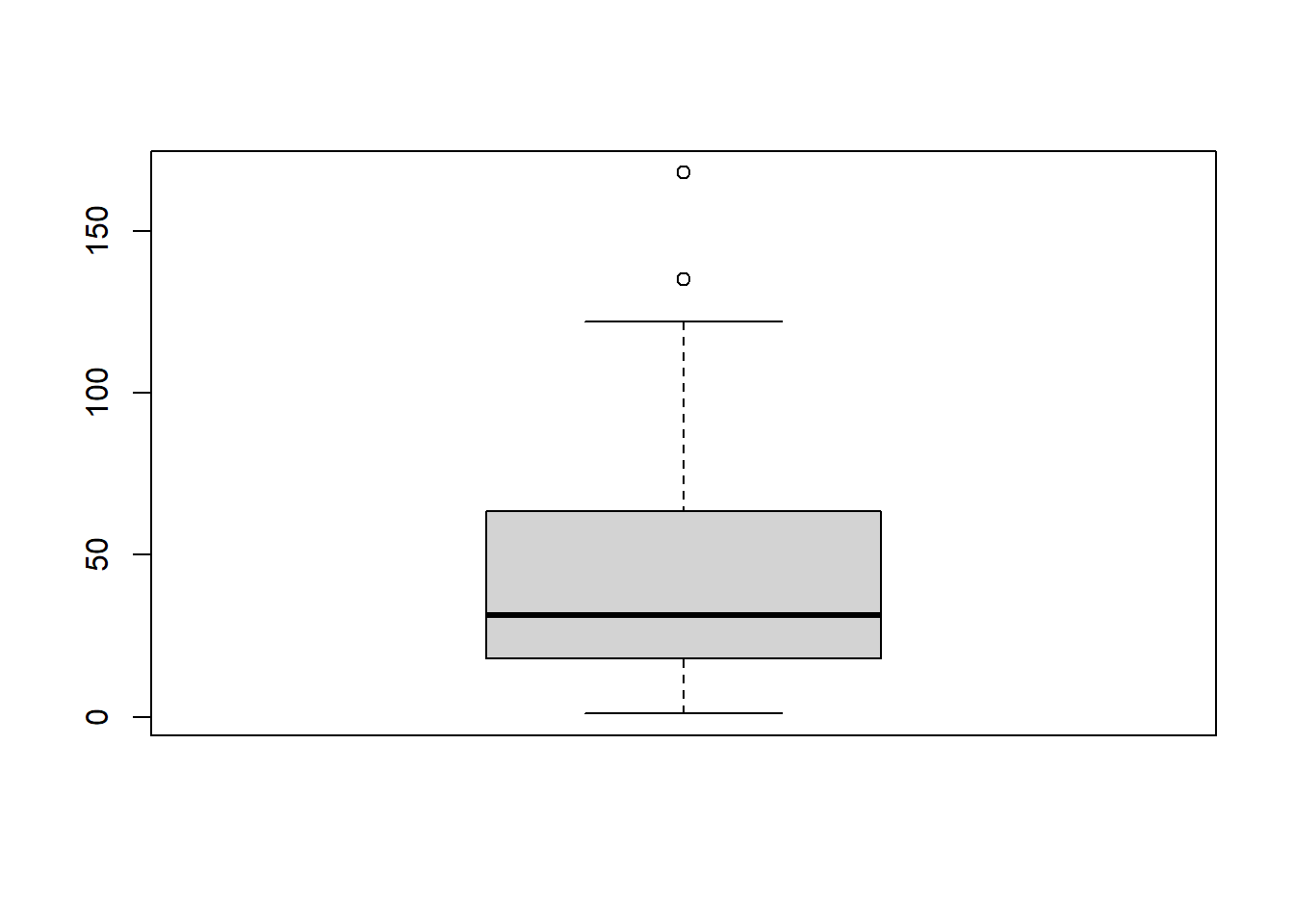
air = airquality # Copy airquality data to temporary storage variable
table(is.na(air$Ozone)) # Check the current number of NAs in Ozone

FALSE  TRUE 
  116    37 
# Change outliers to NA
air$Ozone = ifelse(air$Ozone<1|air$Ozone>122, NA, air$Ozone)
table(is.na(air$Ozone)) # Check the number of NAs after processing outliers (increased by 2)

FALSE  TRUE 
  114    39 
# Remove NA
air_narm = air[!is.na(air$Ozone), ]
mean(air_narm$Ozone) # By removing two outliers, the value is reduced compared to the result using the is.na function.
[1] 40.2

Class


load("data/List_KMP.RData")
names(List.KMP) <- c("p17", "p18", "p19", "d19")
p17_df <- List.KMP[["p17"]]
p18_df <- List.KMP[["p18"]]
p19_df <- List.KMP[["p19"]]


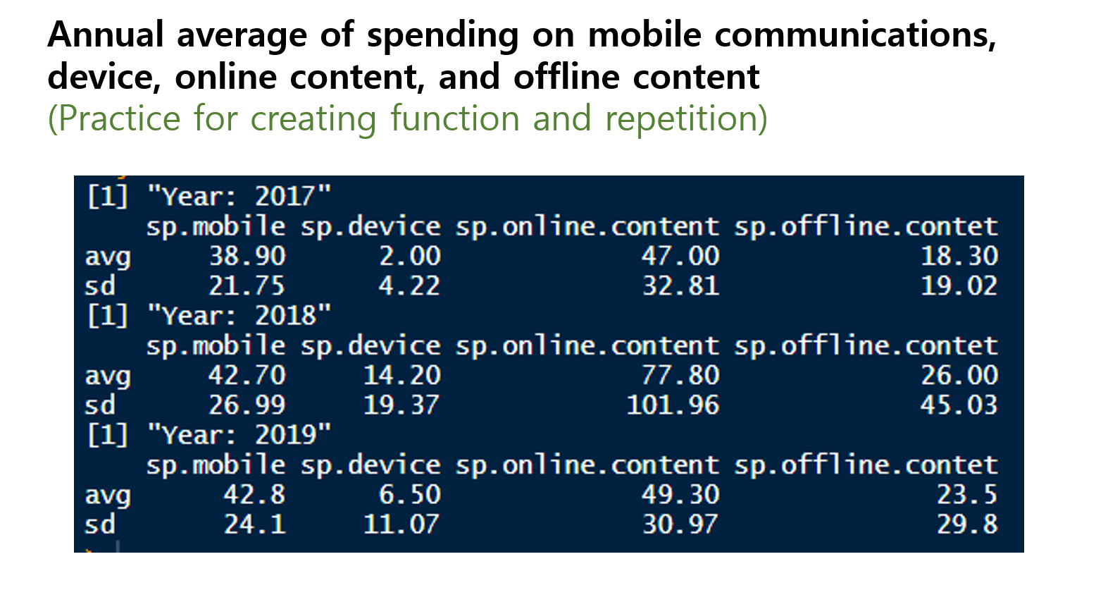
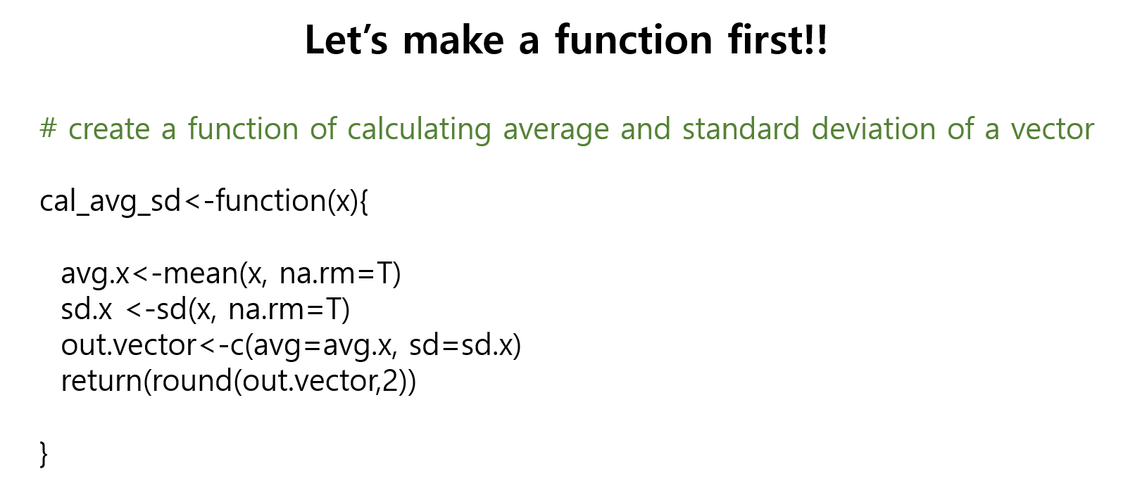
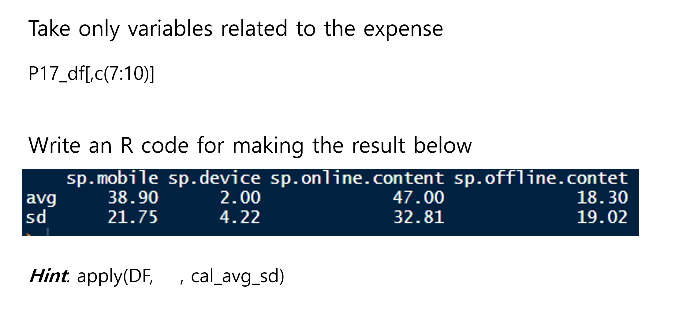
# create a function of calculating average and standard deviation of a vector

cal_avg_sd<-function(x){

  avg.x<-mean(x, na.rm=T)
  sd.x <-sd(x, na.rm=T)
  out.vector<-c(avg=avg.x, sd=sd.x)
  return(round(out.vector,2))

}

Let’s apply this function to dataset ‘p17’

# Let's try this function
cal_avg_sd(p17_df$sp.mobile)
 avg   sd 
38.9 21.8 


Loop, Function, and Data Manipulation in R: A Dive into the Palmer Penguin Dataset

In the world of data analysis with R, mastering the basics of loops, functions, and data manipulation is essential for any aspiring data scientist. While the tidyverse collection of packages offers powerful tools for these tasks, it’s crucial to first understand the foundational techniques that underpin effective data analysis. This week, we embark on a journey with the Palmer Penguin dataset, focusing on traditional R approaches, saving the tidyverse exploration for our next installment.

The Palmer Penguin Dataset: A Brief History

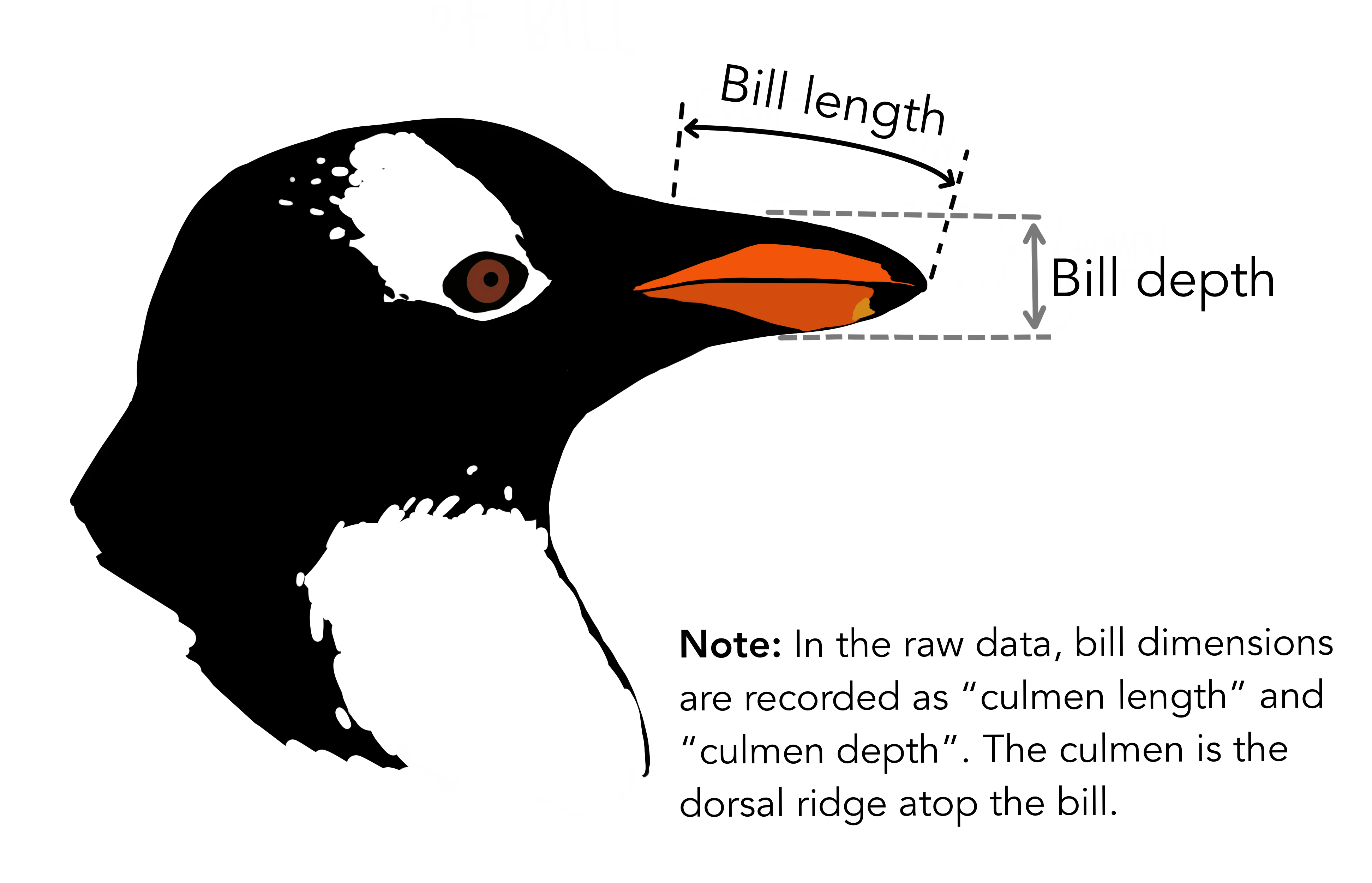
The Palmer Penguin dataset, introduced by Dr. Kristen Gorman and the Palmer Station, Antarctica LTER, provides a compelling alternative to the classic Iris dataset for data exploration and visualization. Comprising data on 344 penguins across three species (Adélie, Gentoo, and Chinstrap) from the Palmer Archipelago in Antarctica, the dataset includes variables such as species, island, bill length and depth, flipper length, body mass, and sex.

This dataset not only offers rich insights into the biological diversity of Antarctic penguins but also serves as an excellent resource for teaching data science techniques due to its manageable size and complexity.

Data Manipulation with Base R

Before diving into complex manipulations, let’s start by loading the Palmer Penguin dataset. Although it’s available through the palmerpenguins package, we’ll keep our focus on base R functions for this exploration.

Loading the Dataset

# Assuming palmerpenguins is installed
library(palmerpenguins)
data("penguins")

With the data loaded, let’s proceed to some basic manipulations using base R functions.

palmerpenguins::penguins
# A tibble: 344 × 8
   species island    bill_length_mm bill_depth_mm flipper_length_mm body_mass_g
   <fct>   <fct>              <dbl>         <dbl>             <int>       <int>
 1 Adelie  Torgersen           39.1          18.7               181        3750
 2 Adelie  Torgersen           39.5          17.4               186        3800
 3 Adelie  Torgersen           40.3          18                 195        3250
 4 Adelie  Torgersen           NA            NA                  NA          NA
 5 Adelie  Torgersen           36.7          19.3               193        3450
 6 Adelie  Torgersen           39.3          20.6               190        3650
 7 Adelie  Torgersen           38.9          17.8               181        3625
 8 Adelie  Torgersen           39.2          19.6               195        4675
 9 Adelie  Torgersen           34.1          18.1               193        3475
10 Adelie  Torgersen           42            20.2               190        4250
# ℹ 334 more rows
# ℹ 2 more variables: sex <fct>, year <int>

See more information on this dataset: https://allisonhorst.github.io/palmerpenguins/


Subsetting Data

Subsetting is crucial for isolating parts of the dataset for analysis. In base R, we can use the subset function or the [ operator.

# Subsetting to include only Adélie penguins
adelie_penguins <- subset(penguins, species == "Adelie")

# Alternatively, using the bracket operator
adelie_penguins <- penguins[penguins$species == "Adelie", ]

Handling Missing Values

Missing data can skew analysis, making its identification and treatment essential.

# Identifying missing values
sum(is.na(penguins))
[1] 19
# Removing rows with any missing value
penguins_clean <- na.omit(penguins)

Creating Custom Functions

Custom functions in R amplify the power of data manipulation by encapsulating repetitive tasks.

# A function to summarize penguin measurements
summarize_measurements <- function(data) {
  summary <- data.frame(
    Mean_FlipperLength = mean(data$flipper_length_mm, na.rm = TRUE),
    SD_FlipperLength = sd(data$flipper_length_mm, na.rm = TRUE),
    Mean_BillLength = mean(data$bill_length_mm, na.rm = TRUE),
    SD_BillLength = sd(data$bill_length_mm, na.rm = TRUE)
  )
  return(summary)
}

# Applying the function to Adélie penguins
adelie_summary <- summarize_measurements(adelie_penguins)
adelie_summary
  Mean_FlipperLength SD_FlipperLength Mean_BillLength SD_BillLength
1                190             6.54            38.8          2.66

Looping Through Data

Loops are essential for iterative operations. In R, for loops allow us to apply operations across elements, rows, or columns in a dataset.

# Calculating mean body mass for each species
species_list <- unique(penguins$species)
# Create an empty vector
mean_mass_by_species <- numeric(0)

for (i in seq_along(species_list)) {
  species_data <- subset(penguins, species == species_list[i])
  mean_mass_by_species[i] <- mean(species_data$body_mass_g, na.rm = TRUE)
}

names(mean_mass_by_species) <- species_list
mean_mass_by_species
   Adelie    Gentoo Chinstrap 
     3701      5076      3733 

This code iterates through each species in the dataset, calculating and storing the mean body mass.

Let’s use customized function instead.

species_list <- unique(penguins$species)
# Create an empty list
summary_by_species <- list(0)

for (i in seq_along(species_list)) {
  species_data <- subset(penguins, species == species_list[i])
  summary_by_species[[i]] <- summarize_measurements(species_data)
}

names(summary_by_species) <- species_list
summary_by_species
$Adelie
  Mean_FlipperLength SD_FlipperLength Mean_BillLength SD_BillLength
1                190             6.54            38.8          2.66

$Gentoo
  Mean_FlipperLength SD_FlipperLength Mean_BillLength SD_BillLength
1                217             6.48            47.5          3.08

$Chinstrap
  Mean_FlipperLength SD_FlipperLength Mean_BillLength SD_BillLength
1                196             7.13            48.8          3.34


Exploration with tidyverse

Let’s enhance our exploration of the Palmer Penguin dataset by paralleling our original code snippets with their tidyverse counterparts. The tidyverse is a collection of R packages designed for data science that makes data manipulation, exploration, and visualization easier and more intuitive.

Loading the Dataset with tidyverse

First, let’s ensure we have the tidyverse and palmerpenguins packages loaded. If you haven’t installed these packages, you can do so using install.packages("tidyverse") and install.packages("palmerpenguins").

library(tidyverse)
── Attaching core tidyverse packages ──────────────────────── tidyverse 2.0.0 ──
✔ dplyr     1.1.3     ✔ readr     2.1.4
✔ forcats   1.0.0     ✔ stringr   1.5.0
✔ ggplot2   3.4.4     ✔ tibble    3.2.1
✔ lubridate 1.9.3     ✔ tidyr     1.3.0
✔ purrr     1.0.2     
── Conflicts ────────────────────────────────────────── tidyverse_conflicts() ──
✖ dplyr::filter() masks stats::filter()
✖ dplyr::lag()    masks stats::lag()
ℹ Use the conflicted package (<http://conflicted.r-lib.org/>) to force all conflicts to become errors
library(palmerpenguins)

Subsetting Data with dplyr

With dplyr, subsetting becomes more readable:

# Subsetting to include only Adélie penguins using dplyr
adelie_penguins <- penguins %>%
  filter(species == "Adelie")

Handling Missing Values with tidyverse

The tidyverse provides a straightforward approach to dealing with missing values:

# Removing rows with any missing value using dplyr
penguins_clean <- penguins %>%
  drop_na()

Creating Custom Functions and Applying them into dataset

While base R functions are powerful, integrating them with tidyverse functionalities can make your workflows even more efficient:

# Using dplyr and purrr to summarize measurements
summarize_measurements <- function(data) {
  data %>%
    summarise(Mean_FlipperLength = mean(flipper_length_mm, na.rm = TRUE),
              SD_FlipperLength = sd(flipper_length_mm, na.rm = TRUE),
              Mean_BillLength = mean(bill_length_mm, na.rm = TRUE),
              SD_BillLength = sd(bill_length_mm, na.rm = TRUE))
}

# Applying the function to Adélie penguins
adelie_summary <- adelie_penguins %>%
  summarize_measurements()
adelie_summary
# A tibble: 1 × 4
  Mean_FlipperLength SD_FlipperLength Mean_BillLength SD_BillLength
               <dbl>            <dbl>           <dbl>         <dbl>
1               190.             6.54            38.8          2.66

Looping Through Data with group_by and summarise

# Calculating mean body mass for each species with dplyr
mean_mass_by_species <- penguins %>%
  group_by(species) %>%
  summarise(MeanBodyMass = mean(body_mass_g, na.rm = TRUE))

mean_mass_by_species
# A tibble: 3 × 2
  species   MeanBodyMass
  <fct>            <dbl>
1 Adelie           3701.
2 Chinstrap        3733.
3 Gentoo           5076.

By incorporating tidyverse techniques, we can make our code more concise and readable, especially for those new to programming or R. The tidyverse syntax is designed to be intuitive, allowing you to more easily understand and articulate what your code is doing, which is particularly beneficial when sharing your work with others or when collaborating on data science projects.


Using purrr for Advanced Data Manipulation

purrr enhances functional programming within the tidyverse ecosystem, providing tools for working effectively with lists and functional programming paradigms. Here’s how we could use purrr in conjunction with dplyr for a task similar to our mean body mass calculation:

Calculating Mean Body Mass by Species with purrr

We can use purrr’s map functions to apply operations across elements in a list, which is particularly useful for more complex or nested operations. While the direct calculation of mean body mass by species is more straightforward with dplyr alone, let’s consider a scenario where purrr demonstrates its utility:

library(tidyverse)
# Splitting the data by species
species_split <- split(penguins, penguins$species)

# Calculating mean body mass for each species using purrr
mean_mass_by_species <- map_dfr(species_split, 
                                ~summarise(.x, MeanBodyMass = mean(body_mass_g, na.rm = TRUE)))

mean_mass_by_species
# A tibble: 3 × 1
  MeanBodyMass
         <dbl>
1        3701.
2        3733.
3        5076.